Question 1

The homoskedasticity-only estimator of the variance of $\hat { \beta }$ 1 is

Accepted Answer

A)  $\frac { s _ { u } ^ { \frac { 2 } { u } } } { \sum _ { i = 1 } ^ { n } \left( X _ { i } - \bar {X } \right) ^ { 2 } }$ 
B)  $\frac { S _ { \hat { u } } ^ { 2 } } { \sqrt { \sum _ { i = 1 } ^ { n } \left( X _ { i } - \bar { X } \right) ^ { 2 } } }$ 
C)  $\frac { S _ { \hat { u } } ^ { 2 } } { \sum _ { i = 1 } ^ { n } X _ { i } ^ { 2 } - \bar { X } } .$ 
D)  $\frac { 1 } { n } \times \frac { \frac { 1 } { n - 2 } \sum _ { i = 1 } ^ { n } \left( X _ { i } - \bar { X } \right) ^ { 2 } \hat { u } _ { i } ^ { 2 } } { \left[ \frac { 1 } { n } \sum _ { i = 1 } ^ { n } \left( X _ { i } - \bar { X } \right) ^ { 2 } \right] ^ { 2 } } { } _ { \times }$ 
A)  $\frac { s _ { u } ^ { \frac { 2 } { u } } } { \sum _ { i = 1 } ^ { n } \left( X _ { i } - \bar {X } \right) ^ { 2 } }$ 
B)  $\frac { S _ { \hat { u } } ^ { 2 } } { \sqrt { \sum _ { i = 1 } ^ { n } \left( X _ { i } - \bar { X } \right) ^ { 2 } } }$ 
C)  $\frac { S _ { \hat { u } } ^ { 2 } } { \sum _ { i = 1 } ^ { n } X _ { i } ^ { 2 } - \bar { X } } .$ 
D)  $\frac { 1 } { n } \times \frac { \frac { 1 } { n - 2 } \sum _ { i = 1 } ^ { n } \left( X _ { i } - \bar { X } \right) ^ { 2 } \hat { u } _ { i } ^ { 2 } } { \left[ \frac { 1 } { n } \sum _ { i = 1 } ^ { n } \left( X _ { i } - \bar { X } \right) ^ { 2 } \right] ^ { 2 } } { } _ { \times }$

Question 2

A binary variable is often called a

Accepted Answer

A) dummy variable. 
B) dependent variable. 
C) residual. 
D) power of a test. 
A) dummy variable. 
B) dependent variable. 
C) residual. 
D) power of a test.

Question 3

Using the California School data set from your textbook, you run the following regression: $\widehat {\text { TestScr }}$ = 698.9 - 2.28 STR
n = 420, SER = 9.4
where TestScore is the average test score in the district and STR is the student-teacher ratio. The sample standard deviation of test scores is 19.05, and the sample standard deviation of the student teacher ratio is 1.89.
a.
Find the regression R2 and the correlation coefficient between test scores and the student teacher ratio.
b.
Find the homoskedasticity-only standard error of the slope.

Accepted Answer

a. R² = 1 - @#LAT-DLM& = 1 - @#LAT-DLM& =

Question 4

(Continuation from Chapter 4, number 6)The neoclassical growth model predicts that for identical savings rates and population growth rates, countries should converge to the per capita income level. This is referred to as the convergence hypothesis. One way to test for the presence of convergence is to compare the growth rates over time to the initial starting level.
(a)The results of the regression for 104 countries were as follows: $\widehat { g 6090 }$  = 0.019 - 0.0006 × RelProd60, R2= 0.00007, SER = 0.016
(0.004)(0.0073)   where g6090 is the average annual growth rate of GDP per worker for the 1960-1990 sample period, and RelProd60 is GDP per worker relative to the United States in 1960. Numbers in parenthesis are heteroskedasticity robust standard errors.
Using the OLS estimator with homoskedasticity-only standard errors, the results changed as follows: $\widehat { g 6090 }$  = 0.019 - 0.0006×RelProd60, R2= 0.00007, SER = 0.016
(0.002)(0.0068)
Why didn't the estimated coefficients change? Given that the standard error of the slope is now smaller, can you reject the null hypothesis of no beta convergence? Are the results in the second equation more reliable than the results in the first equation? Explain.
(b)You decide to restrict yourself to the 24 OECD countries in the sample. This changes your regression output as follows (numbers in parenthesis are heteroskedasticity robust standard errors): $\widehat { g 6090 }$ = 0.048 - 0.0404 RelProd60, R2 = 0.82, SER = 0.0046
(0.004)(0.0063)
Test for evidence of convergence now. If your conclusion is different than in (a), speculate why this is the case.
(c)The authors of your textbook have informed you that unless you have more than 100 observations, it may not be plausible to assume that the distribution of your OLS estimators is normal. What are the implications here for testing the significance of your theory?

Accepted Answer

(a)Using homoskedasticity-only standard

Question 5

Heteroskedasticity means that

Accepted Answer

A) homogeneity cannot be assumed automatically for the model. 
B) the variance of the error term is not constant. 
C) the observed units have different preferences. 
D) agents are not all rational. 
A) homogeneity cannot be assumed automatically for the model. 
B) the variance of the error term is not constant. 
C) the observed units have different preferences. 
D) agents are not all rational.

Question 6

Using 143 observations, assume that you had estimated a simple regression function and that your estimate for the slope was 0.04, with a standard error of 0.01. You want to test whether or not the estimate is statistically significant. Which of the following possible decisions is the only correct one:

Accepted Answer

A) you decide that the coefficient is small and hence most likely is zero in the population 
B) the slope is statistically significant since it is four standard errors away from zero 
C) the response of Y given a change in X must be economically important since it is statistically significant 
D) since the slope is very small, so must be the regression R2. 
A) you decide that the coefficient is small and hence most likely is zero in the population 
B) the slope is statistically significant since it is four standard errors away from zero 
C) the response of Y given a change in X must be economically important since it is statistically significant 
D) since the slope is very small, so must be the regression R2.

Question 7

Let $u _ { i }$ be distributed N(0, $\sigma _ { u } ^ { 2 }$ ), i.e., the errors are distributed normally with a constant variance (homoskedasticity). This results in $\hat{\beta }_ { 1 }$ being distributed N(?1, $\sigma _ { \hat { \beta } 1 } ^ { 2 }$ ), where $\sigma _ { p 1 } ^ { 2 } = \frac { \sigma _ { u } ^ { 2 } } { \sum _ { i = 1 } ^ { n } \left( X _ { i } - \bar { X } \right) ^ { 2 } }$ Statistical inference would be straightforward if $\sigma _ { u } ^ { 2 }$ was known. One way to deal with this problem is to replace $\sigma _ { u } ^ { 2 }$ with an estimator $S _ { \hat { u} } ^ { 2 }$ Clearly since this introduces more uncertainty, you cannot expect $\hat{\beta} _ { 1 }$ to be still normally distributed. Indeed, the t-statistic now follows Student's t distribution. Look at the table for the Student t-distribution and focus on the 5% two-sided significance level. List the critical values for 10 degrees of freedom, 30 degrees of freedom, 60 degrees of freedom, and finally ? degrees of freedom. Describe how the notion of uncertainty about $\sigma _ { u } ^ { 2 }$ can be incorporated about the tails of the t-distribution as the degrees of freedom increase.

Accepted Answer

More uncertainty implies that the tales

Question 8

You extract approximately 5,000 observations from the Current Population Survey (CPS)and estimate the following regression function: $\widehat { \text { ahe } }$ = 3.32 - 0.45 $\times$ Age, R2= 0.02, SER = 8.66 (1.00)(0.04)
Where ahe is average hourly earnings, and Age is the individual's age. Given the specification, your 95% confidence interval for the effect of changing age by 5 years is approximately

Accepted Answer

A) [$1.96, $2.54] 
B) [$2.32, $4.32] 
C) [$1.35, $5.30] 
D) cannot be determined given the information provided 
A) [$1.96, $2.54] 
B) [$2.32, $4.32] 
C) [$1.35, $5.30] 
D) cannot be determined given the information provided

Question 9

Using the California School data set from your textbook, you run the following regression: $\widehat {\text { TestScr} }$ = 698.9 - 2.28 STR
n = 420, R2 = 0.051, SER = 18.6
where TestScore is the average test score in the district and STR is the student-teacher ratio. Using heteroskedasticity robust standard errors, you find $\hat { \sigma } _ { \hat { \beta} _ { 1 }  } = 0.52$ while choosing the homoskedasticity-only option, the standard error is 0.48.
a. Calculate the t-statistic for both standard errors.
b. Which of the two t-statistics should you base your inference on?

Accepted Answer

a. The respective t-statistics are 4.39

Question 10

One of the following steps is not required as a step to test for the null hypothesis:

Accepted Answer

A) compute the standard error of $\hat { \beta }$ 1. 
B) test for the errors to be normally distributed. 
C) compute the t-statistic. 
D) compute the p-value. 
A) compute the standard error of $\hat { \beta }$ 1. 
B) test for the errors to be normally distributed. 
C) compute the t-statistic. 
D) compute the p-value.

Question 11

(Continuation of the Purchasing Power Parity question from Chapter 4)The news-magazine The Economist regularly publishes data on the so called Big Mac index and exchange rates between countries. The data for 30 countries from the April 29, 2000 issue is listed below:
 
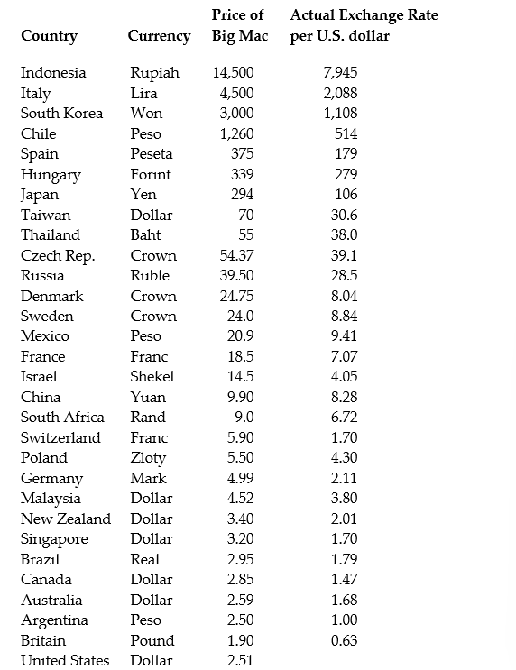The concept of purchasing power parity or PPP ("the idea that similar foreign and domestic goods … should have the same price in terms of the same currency," Abel, A. and B. Bernanke, Macroeconomics, 4th edition, Boston: Addison Wesley, 476)suggests that the ratio of the Big Mac priced in the local currency to the U.S. dollar price should equal the exchange rate between the two countries.
After entering the data into your spread sheet program, you calculate the predicted exchange rate per U.S. dollar by dividing the price of a Big Mac in local currency by the U.S. price of a Big Mac ($2.51). To test for PPP, you regress the actual exchange rate on the predicted exchange rate.
The estimated regression is as follows: $\widehat{\text { ActualExRate }}$ = -27.05 + 1.35 × 1.35×Pr edExRate R2 = 0.994, n = 29, SER = 122.15
(23.74)(0.02)
(a)Your spreadsheet program does not allow you to calculate heteroskedasticity robust standard errors. Instead, the numbers in parenthesis are homoskedasticity only standard errors. State the two null hypothesis under which PPP holds. Should you use a one-tailed or two-tailed alternative hypothesis?
(b)Calculate the two t-statistics.
(c)Using a 5% significance level, what is your decision regarding the null hypothesis given the two t-statistics? What critical values did you use? Are you concerned with the fact that you are testing the two hypothesis sequentially when they are supposed to hold simultaneously?
(d)What assumptions had to be made for you to use Student's t-distribution?

Accepted Answer

(a)Under PPP, H₀ : ?₀ = 0 and H_o : ?₁ = 1. E

Question 12

Imagine that you were told that the t-statistic for the slope coefficient of the regression line $\widehat {\text { TestScore }}$ = 698.9 - 2.28 × STR was 4.38. What are the units of measurement for the t-statistic?

Accepted Answer

A) points of the test score 
B) number of students per teacher 
C)  $\frac { \text { TestScore } } { S T R }$ 
D) standard deviations 
A) points of the test score 
B) number of students per teacher 
C)  $\frac { \text { TestScore } } { S T R }$ 
D) standard deviations

Question 13

In general, the t-statistic has the following form:

Accepted Answer

A)  $\frac{\text {estimate-hypothesize value }}{\text { standard error of estimate}}$ 
B)  $\frac{\text {estimator }}{\text {standard error of estimate }}$ 
C)  $\frac{\text {estimator-hypothesize value  }}{\text { standard error of estimate}}$ 
D)  $\frac { \frac { \text { estimator - hypothesize value } } { \text { standard error of estimator } } } { \sqrt { n } }$ 
A)  $\frac{\text {estimate-hypothesize value }}{\text { standard error of estimate}}$ 
B)  $\frac{\text {estimator }}{\text {standard error of estimate }}$ 
C)  $\frac{\text {estimator-hypothesize value  }}{\text { standard error of estimate}}$ 
D)  $\frac { \frac { \text { estimator - hypothesize value } } { \text { standard error of estimator } } } { \sqrt { n } }$

Question 14

When estimating a demand function for a good where quantity demanded is a linear function of the price, you should

Accepted Answer

A) not include an intercept because the price of the good is never zero. 
B) use a one-sided alternative hypothesis to check the influence of price on quantity. 
C) use a two-sided alternative hypothesis to check the influence of price on quantity. 
D) reject the idea that price determines demand unless the coefficient is at least 1.96. 
A) not include an intercept because the price of the good is never zero. 
B) use a one-sided alternative hypothesis to check the influence of price on quantity. 
C) use a two-sided alternative hypothesis to check the influence of price on quantity. 
D) reject the idea that price determines demand unless the coefficient is at least 1.96.

Question 15

The t-statistic is calculated by dividing

Accepted Answer

A) the OLS estimator by its standard error. 
B) the slope by the standard deviation of the explanatory variable. 
C) the estimator minus its hypothesized value by the standard error of the estimator. 
D) the slope by 1.96. 
A) the OLS estimator by its standard error. 
B) the slope by the standard deviation of the explanatory variable. 
C) the estimator minus its hypothesized value by the standard error of the estimator. 
D) the slope by 1.96.

Question 16

You have collected data for the 50 U.S. states and estimated the following relationship between the change in the unemployment rate from the previous year ( $\widehat{\Delta u r}$ )and the growth rate of the respective state real GDP (gy). The results are as follows $\widehat{\Delta u r}$ = 2.81 - 0.23 $\times$ gy, R2= 0.36, SER = 0.78 (0.12)(0.04)
Assuming that the estimator has a normal distribution, the 95% confidence interval for the slope is approximately the interval

Accepted Answer

A) [2.57, 3.05] 
B) [-0.31,0.15] 
C) [-0.31, -0.15] 
D) [-0.33, -0.13] 
A) [2.57, 3.05] 
B) [-0.31,0.15] 
C) [-0.31, -0.15] 
D) [-0.33, -0.13]

Question 17

Assume that your population regression function is
Yi = ?iXi + ui
i.e., a regression through the origin (no intercept). Under the homoskedastic normal regression assumptions, the t-statistic will have a Student t distribution with n-1 degrees of freedom, not n-2 degrees of freedom, as was the case in Chapter 5 of your textbook. Explain. Do you think that the residuals will still sum to zero for this case?

Accepted Answer

In deriving the OLS estimator @#LAT-DLM& ₁, you min

Question 18

The effect of decreasing the student-teacher ratio by one is estimated to result in an improvement of the districtwide score by 2.28 with a standard error of 0.52. Construct a 90% and 99% confidence interval for the size of the slope coefficient and the corresponding predicted effect of changing the student-teacher ratio by one. What is the intuition on why the 99% confidence interval is wider than the 90% confidence interval?

Accepted Answer

The 90% confidence interval for the slop

Question 19

Below you are asked to decide on whether or not to use a one-sided alternative or a two-sided alternative hypothesis for the slope coefficient. Briefly justify your decision.
(a) $\hat { q } _ { i } ^ { d }$ = $\hat { \beta }$ 0 + $\hat { \beta }$ 1pi, where qd is the quantity demanded for a good, and p is its price.
(b) $\hat { p } _ { i } ^ { actual}$ = $\hat { \beta }$ 0 + $\hat { \beta }$ 1
  $\hat { p } _ { i } ^ { actual}$ , where $\hat { p } _ { i } ^ { actual}$ is the actual house price, and $\hat { p } _ { i } ^ { actual}$ is the assessed house price. You want to test whether or not the assessment is correct, on average.
(c) $\hat { C }$ i = $\hat { \beta }$ 0 + $\hat { \beta }$ 1
  $Y _ { i } ^ { d }$ , where C is household consumption, and Yd is personal disposable income.

Accepted Answer

(a)You would use a one-sided alternative

The homoskedasticity-only estimator of the variance of $\hat { \beta }$ ₁ is

A binary variable is often called a

Heteroskedasticity means that

One of the following steps is not required as a step to test for the null hypothesis:

Imagine that you were told that the t-statistic for the slope coefficient of the regression line $\widehat {\text { TestScore }}$ = 698.9 - 2.28 × STR was 4.38. What are the units of measurement for the t-statistic?

In general, the t-statistic has the following form:

When estimating a demand function for a good where quantity demanded is a linear function of the price, you should

The t-statistic is calculated by dividing

Economic Questions and Data

Review of Probability

Review of Statistics

Linear Regression With One Regressor

Linear Regression With Multiple Regressors

Hypothesis Tests and Confidence Intervals in Multiple Regression

Nonlinear Regression Functions

Assessing Studies Based on Multiple Regression

Regression With Panel Data

Regression With a Binary Dependent Variable

Instrumental Variables Regression

Experiments and Quasi-Experiments

Introduction to Time Series Regression and Forecasting

Estimation of Dynamic Causal Effects

Additional Topics in Time Series Regression

The Theory of Linear Regression With One Regressor

The Theory of Multiple Regression

Filters

Exam 5: Regression With a Single Regressor: Hypothesis Tests and Confidence Intervals

The homoskedasticity-only estimator of the variance of β^\hat { \beta }β^​ 1 is

A binary variable is often called a

Heteroskedasticity means that

One of the following steps is not required as a step to test for the null hypothesis:

Imagine that you were told that the t-statistic for the slope coefficient of the regression line TestScore ^\widehat {\text { TestScore }} TestScore = 698.9 - 2.28 × STR was 4.38. What are the units of measurement for the t-statistic?

In general, the t-statistic has the following form:

When estimating a demand function for a good where quantity demanded is a linear function of the price, you should

The t-statistic is calculated by dividing

Economic Questions and Data

Review of Probability

Review of Statistics

Linear Regression With One Regressor

Linear Regression With Multiple Regressors

Hypothesis Tests and Confidence Intervals in Multiple Regression

Nonlinear Regression Functions

Assessing Studies Based on Multiple Regression

Regression With Panel Data

Regression With a Binary Dependent Variable

Instrumental Variables Regression

Experiments and Quasi-Experiments

Introduction to Time Series Regression and Forecasting

Estimation of Dynamic Causal Effects

Additional Topics in Time Series Regression

The Theory of Linear Regression With One Regressor

The Theory of Multiple Regression

Filters

The homoskedasticity-only estimator of the variance of $\hat { \beta }$ ₁ is

Imagine that you were told that the t-statistic for the slope coefficient of the regression line $\widehat {\text { TestScore }}$ = 698.9 - 2.28 × STR was 4.38. What are the units of measurement for the t-statistic?