Exam 14: Introduction to Time Series Regression and Forecasting
Exam 1: Economic Questions and Data17 Questions
Exam 2: Review of Probability70 Questions
Exam 3: Review of Statistics65 Questions
Exam 4: Linear Regression With One Regressor65 Questions
Exam 5: Regression With a Single Regressor: Hypothesis Tests and Confidence Intervals59 Questions
Exam 6: Linear Regression With Multiple Regressors65 Questions
Exam 7: Hypothesis Tests and Confidence Intervals in Multiple Regression64 Questions
Exam 8: Nonlinear Regression Functions63 Questions
Exam 9: Assessing Studies Based on Multiple Regression65 Questions
Exam 10: Regression With Panel Data50 Questions
Exam 11: Regression With a Binary Dependent Variable50 Questions
Exam 12: Instrumental Variables Regression50 Questions
Exam 13: Experiments and Quasi-Experiments50 Questions
Exam 14: Introduction to Time Series Regression and Forecasting50 Questions
Exam 15: Estimation of Dynamic Causal Effects50 Questions
Exam 16: Additional Topics in Time Series Regression50 Questions
Exam 17: The Theory of Linear Regression With One Regressor49 Questions
Exam 18: The Theory of Multiple Regression50 Questions
Select questions type
You should use the QLR test for breaks in the regression coefficients, when
(Multiple Choice)
4.9/5  (38)
(38)
The Akaike Information Criterion (AIC)is given by the following formula
(Multiple Choice)
4.8/5 (39)
If a "break" occurs in the population regression function, then
(Multiple Choice)
4.9/5 (35)
The textbook displayed the accompanying four economic time series with "markedly different patterns." For each indicate what you think the sample autocorrelations of the level (Y)and change (△Y)will be and explain your reasoning.
(a) 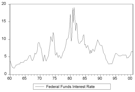 (b)
(b) 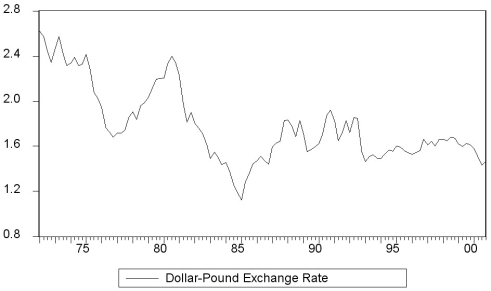 (c)
(c) 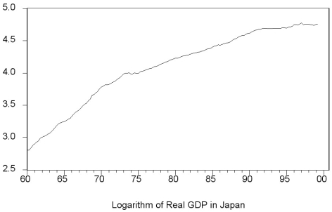 (d)
(d) 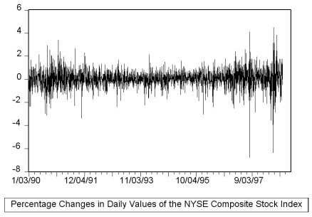
(Essay)
4.8/5 (40)
Problems caused by stochastic trends include all of the following with the exception of
(Multiple Choice)
4.8/5 (36)
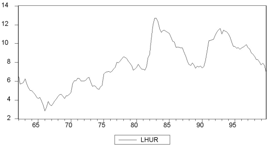
There is some evidence that the Phillips curve has been unstable during the 1962 to 1999 period for the United States, and in particular during the 1990s. You set out to investigate whether or not this instability also occurred in other places. Canada is a particularly interesting case, due to its proximity to the United States and the fact that many features of its economy are similar to that of the U.S.
(a)Reading up on some of the comparative economic performance literature, you find that Canadian unemployment rates were roughly the same as U.S. unemployment rates from the 1920s to the early 1980s. The accompanying figure shows that a gap opened between the unemployment rates of the two countries in 1982, which has persisted to this date. 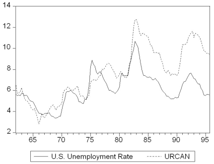 Inspection of the graph and data suggest that the break occurred during the second quarter of 1982. To investigate whether the Canadian Phillips curve shows a break at that point, you estimate an ADL(4,4)model for the sample period 1962:I-1999:IV and perform a Chow test. Specifically you postulate that the constant and coefficients of the unemployment rates changed at that point. The F-statistic is 1.96. Find the critical value from the F-table and test the null hypothesis that a break occurred at that time. Is there any reason why you should be skeptical about the result regarding the break and using the Chow-test to detect it?
(b)You consider alternative ways to test for a break in the relationship. The accompanying figure shows the F-statistics testing for a break in the ADL(4,4)equation at different dates.
Inspection of the graph and data suggest that the break occurred during the second quarter of 1982. To investigate whether the Canadian Phillips curve shows a break at that point, you estimate an ADL(4,4)model for the sample period 1962:I-1999:IV and perform a Chow test. Specifically you postulate that the constant and coefficients of the unemployment rates changed at that point. The F-statistic is 1.96. Find the critical value from the F-table and test the null hypothesis that a break occurred at that time. Is there any reason why you should be skeptical about the result regarding the break and using the Chow-test to detect it?
(b)You consider alternative ways to test for a break in the relationship. The accompanying figure shows the F-statistics testing for a break in the ADL(4,4)equation at different dates. 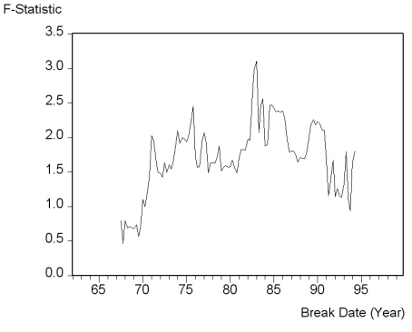 The QLR-statistic with 15% trimming is 3.11. Comment on the figure and test for the hypothesis of a break in the ADL(4,4)regression.
(c)To test for the stability of the Canadian Phillips curve in the 1990s, you decide to perform a pseudo out-of-sample forecasting. For the 24 quarters from 1994:I-1999:IV you use the ADL(4,4)model to calculate the forecasted change in the inflation rate, the resulting forecasted inflation rate, and the forecast error. The standard error of the ADL(4,4)for the estimation sample period 1962:1-1993:4 is 1.91 and the sample RMSFE is 1.70. The average forecast error for the 24 inflation rates is 0.003 and the sample standard deviation of the forecast errors is 0.82. Calculate the t-statistic and test the hypothesis that the mean out-of-sample forecast error is zero. Comment on the result and the accompanying figure of the actual and forecasted inflation rate.
The QLR-statistic with 15% trimming is 3.11. Comment on the figure and test for the hypothesis of a break in the ADL(4,4)regression.
(c)To test for the stability of the Canadian Phillips curve in the 1990s, you decide to perform a pseudo out-of-sample forecasting. For the 24 quarters from 1994:I-1999:IV you use the ADL(4,4)model to calculate the forecasted change in the inflation rate, the resulting forecasted inflation rate, and the forecast error. The standard error of the ADL(4,4)for the estimation sample period 1962:1-1993:4 is 1.91 and the sample RMSFE is 1.70. The average forecast error for the 24 inflation rates is 0.003 and the sample standard deviation of the forecast errors is 0.82. Calculate the t-statistic and test the hypothesis that the mean out-of-sample forecast error is zero. Comment on the result and the accompanying figure of the actual and forecasted inflation rate. 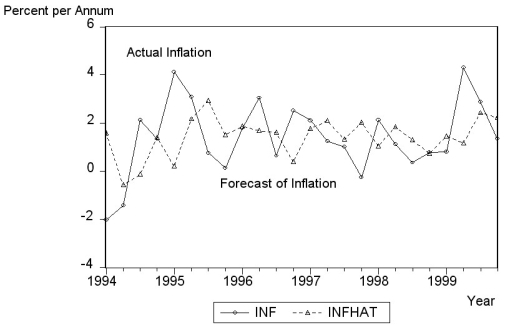
(Essay)
4.9/5 (41)
You collect monthly data on the money supply (M2)for the United States from 1962:1-2002:4 to forecast future money supply behavior. 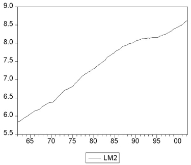
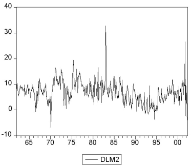 where LM2 and DLM2 are the log level and growth rate of M2.
(a)Using quarterly data, when analyzing inflation and unemployment in the United States, the textbook converted log levels of variables into growth rates by differencing the log levels, and then multiplying these by 400. Given that you have monthly data, how would you proceed here?
(b)How would you go about testing for a stochastic trend in LM2 and DLM2? Be specific about how to decide the number of lags to be included and whether or not to include a deterministic trend in your test. The textbook found the (quarterly)inflation rate to have a unit root. Does this have any affect on your expectation about whether or not the (monthly)money growth rate should be stationary?
(c)You decide to conduct an ADF unit root test for LM2, DLM2, and the change in the growth rate ΔDLM2. This results in the following t-statistic on the parameter of interest. LM2 with trend DLM2 without trend DLM2 with trend \triangleDLM2 without trend -0.505 -4.100 -4.592 -8.897 Find the critical value at the 1%, 5%, and 10% level and decide which of the coefficients is significant. What is the alternative hypothesis?
(d)In forecasting the money growth rate, you add lags of the monetary base growth rate (DLMB)to see if you can improve on the forecasting performance of a chosen AR(10)model in DLM2. You perform a Granger causality test on the 9 lags of DLMB and find a F-statistic of 2.31. Discuss the implications.
(e)Curious about the result in the previous question, you decide to estimate an ADL(10,10)for DLMB and calculate the F-statistic for the Granger causality test on the 9 lag coefficients of DLM2. This turns out to be 0.66. Discuss.
(f)Is there any a priori reason for you to be skeptical of the results? What other tests should you perform?
where LM2 and DLM2 are the log level and growth rate of M2.
(a)Using quarterly data, when analyzing inflation and unemployment in the United States, the textbook converted log levels of variables into growth rates by differencing the log levels, and then multiplying these by 400. Given that you have monthly data, how would you proceed here?
(b)How would you go about testing for a stochastic trend in LM2 and DLM2? Be specific about how to decide the number of lags to be included and whether or not to include a deterministic trend in your test. The textbook found the (quarterly)inflation rate to have a unit root. Does this have any affect on your expectation about whether or not the (monthly)money growth rate should be stationary?
(c)You decide to conduct an ADF unit root test for LM2, DLM2, and the change in the growth rate ΔDLM2. This results in the following t-statistic on the parameter of interest. LM2 with trend DLM2 without trend DLM2 with trend \triangleDLM2 without trend -0.505 -4.100 -4.592 -8.897 Find the critical value at the 1%, 5%, and 10% level and decide which of the coefficients is significant. What is the alternative hypothesis?
(d)In forecasting the money growth rate, you add lags of the monetary base growth rate (DLMB)to see if you can improve on the forecasting performance of a chosen AR(10)model in DLM2. You perform a Granger causality test on the 9 lags of DLMB and find a F-statistic of 2.31. Discuss the implications.
(e)Curious about the result in the previous question, you decide to estimate an ADL(10,10)for DLMB and calculate the F-statistic for the Granger causality test on the 9 lag coefficients of DLM2. This turns out to be 0.66. Discuss.
(f)Is there any a priori reason for you to be skeptical of the results? What other tests should you perform?
(Essay)
4.8/5 (39)
(Requires Internet access for the test question)
The following question requires you to download data from the internet and to load it into a statistical package such as STATA or EViews.
a. Your textbook suggests using two test statistics to test for stationarity: DF and ADF. Test the null hypothesis that inflation has a stochastic trend against the alternative that it is stationary by performing the DF and ADF test for a unit autoregressive root. That is, use the equation (14.34)in your textbook with four lags and without a lag of the change in the inflation rate as a regressor for sample period 1962:I - 2004:IV. Go to the Stock and Watson companion website for the textbook and download the data "Macroeconomic Data Used in Chapters 14 and 16." Enter the data for consumer price index, calculate the inflation rate and the acceleration of the inflation rate, and replicate the result on page 526 of your textbook. Make sure not to use the heteroskedasticity-robust standard error option for the estimation.
b. Next find a website with more recent data, such as the Federal Reserve Economic Data (FRED)site at the Federal Reserve Bank of St. Louis. Locate the data for the CPI, which will be monthly, and convert the data in quarterly averages. Then, using a sample from 1962:I - 2009:IV, re-estimate the above specification and comment on the changes that have occurred.
c. For the new sample period, find the DF statistic.
d. Finally, calculate the ADF statistic, allowing for the lag length of the inflation acceleration term to be determined by either the AIC or the BIC.
(Essay)
4.7/5 (33)
You set out to forecast the unemployment rate in the United States (UrateUS), using quarterly data from 1960, first quarter, to 1999, fourth quarter.
(a)The following table presents the first four autocorrelations for the United States aggregate unemployment rate and its change for the time period 1960 (first quarter)to 1999 (fourth quarter). Explain briefly what these two autocorrelations measure.
First Four Autocorrelations of the U.S. Unemployment Rate and Its Change,
1960:I - 1999:IV Lag Unemployment Rate Change of Unemployment Rate 1 0.97 0.62 2 0.92 0.32 3 0.83 0.12 4 0.75 -0.07 (b)The accompanying table gives changes in the United States aggregate unemployment rate for the period 1999:I-2000:I and levels of the current and lagged unemployment rates for 1999:I. Fill in the blanks for the missing unemployment rate levels.
Changes in Unemployment Rates in the United States
First Quarter 1999 to First Quarter 2000 Quarter U.S. Unemployment Rate First Lag Change in Unemployment Rate 1999:I 4.3 4.4 -0.1 1999: II 0.0 1999:III -0.1 1999:IV -0.1 2000:I -0.1 (c)You decide to estimate an AR(1)in the change in the United States unemployment rate to forecast the aggregate unemployment rate. The result is as follows: = -0.003 + 0.621 ? UrateUSt-1, R2 = 0.393, SER = 0.255
(0.022)(0.106)
The AR(1)coefficient for the change in the inflation rate was 0.211 and the regression R2 was 0.04. What does the difference in the results suggest here?
(d)The textbook used the change in the log of the price level to approximate the inflation rate, and then predicted the change in the inflation rate. Why aren't logarithms used here?
(e)If much of the forecast error arises as a result of future error terms dominating the error resulting from estimating the unknown coefficients, then what is your best guess of the RMSFE here?
(f)The actual unemployment rate during the fourth quarter of 1999 is 4.1 percent, and it decreased from the third quarter to the fourth quarter by 0.1 percent. What is your forecast for the unemployment rate level in the first quarter of 1996?
(g)You want to see how sensitive your forecast is to changes in the specification. Given that you have estimated the regression with quarterly data, you consider an AR(4)model. This results in the following output =-0.005+0.663\Delta-0.082 (0.022)(0.125)(0.139)
What is your forecast for the unemployment rate level in 2000:I? Compare the forecast error of the AR(4)model with the forecast error of the AR(1)model.
(h)There does not seem to be much difference in the forecast of the unemployment rate level, whether you use the AR(1)or the AR(4). Given the various information criteria and the regression R2 below, which model should you use for forecasting?
2 0 0.604 0.624 0.000 1 0.158 0.1181 0.393 2 0.185 0.125 0.397 3 0.217 0.138 0.400 4 0.218 0.1183 0.416 5 0.249 0.130 0.417 6 0.277 0.138 0.420
(Essay)
4.8/5 (39)
(Requires Internet Access for the test question)
The following question requires you to download data from the internet and to load it into a statistical package such as STATA or EViews.
a. Your textbook estimates an AR(1)model (equation 14.7)for the change in the inflation rate using a sample period 1962:I - 2004:IV. Go to the Stock and Watson companion website for the textbook and download the data "Macroeconomic Data Used in Chapters 14 and 16." Enter the data for consumer price index, calculate the inflation rate, the acceleration of the inflation rate, and replicate the result on page 526 of your textbook. Make sure to use heteroskedasticity-robust standard error option for the estimation.
b. Next find a website with more recent data, such as the Federal Reserve Economic Data (FRED)site at the Federal Reserve Bank of St. Louis. Locate the data for the CPI, which will be monthly, and convert the data in quarterly averages. Then, using a sample from 1962:I - 2009:IV, re-estimate the above specification and comment on the changes that have occurred.
c. Based on the BIC, how many lags should be included in the forecasting equation for the change in the inflation rate? Use the new data set and sample period to answer the question.
(Essay)
4.8/5 (37)
Having learned in macroeconomics that consumption depends on disposable income, you want to determine whether or not disposable income helps predict future consumption. You collect data for the sample period 1962:I to 1995:IV and plot the two variables.
(a)To determine whether or not past values of personal disposable income growth rates help to predict consumption growth rates, you estimate the following relationship. t=1.695+0.126\DeltaLn+0.153\DeltaLn , (0.484) (0.099) (0.103) +0.294\DeltaLn-0.008\DeltaLn (0.103) (0.102) +0.088\DeltaLn-0.031\DeltaLn-0.050\DeltaLn-0.091\Delta Ln (0.076)(0.078)(0.078)(0.074)
The Granger causality test for the exclusion on all four lags of the GDP growth rate is 0.98. Find the critical value for the 1%, the 5%, and the 10% level from the relevant table and make a decision on whether or not these additional variables Granger cause the change in the growth rate of consumption.
(b)You are somewhat surprised about the result in the previous question and wonder, how sensitive it is with regard to the lag length in the ADL(p,q)model. As a result, you calculate BIC and AIC of p and q from 0 to 6. The results are displayed in the accompanying table: p,q BIC AIC 0 5.061 5.039 1 5.052 4.988 2 5.095 4.989 3 5.110 4.960 4 5.165 4.972 5 5.206 4.973 6 5.270 4.992 Which values for p and q should you choose?
(c)Estimating an ADL(1,1)model gives you a t-statistic of 1.28 on the coefficient of lagged disposable income growth. What does the Granger causality test suggest about the inclusion of lagged income growth as a predictor of consumption growth?
(Essay)
4.8/5 (42)
You have collected quarterly data on Canadian unemployment (UrateC)and inflation (InfC)from 1962 to 1999 with the aim to forecast Canadian inflation.
(a)To get a better feel for the data, you first inspect the plots for the series. 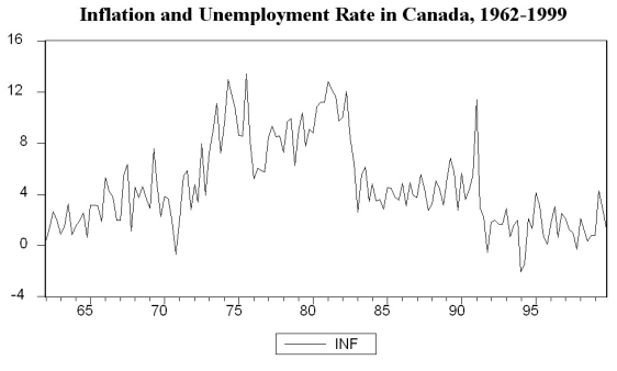
 Inspecting the Canadian inflation rate plot and having calculated the first autocorrelation to be 0.79 for the sample period, do you suspect that the Canadian inflation rate has a stochastic trend? What more formal methods do you have available to test for a unit root?
(b)You run the following regression, where the numbers in parenthesis are homoskedasticity-only standard errors:
(0.28)(0.05) (0.09) (0.09) (0.09) (0.08)
Test for the presence of a stochastic trend. Should you have used heteroskedasticity-robust standard errors? Does the fact that you use quarterly data suggest including four lags in the above regression, or how should you determine the number of lags?
(c)To forecast the Canadian inflation rate for 2000:I, you estimate an AR(1), AR(4), and an ADL(4,1)model for the sample period 1962:I to 1999:IV. The results are as follows:
Inspecting the Canadian inflation rate plot and having calculated the first autocorrelation to be 0.79 for the sample period, do you suspect that the Canadian inflation rate has a stochastic trend? What more formal methods do you have available to test for a unit root?
(b)You run the following regression, where the numbers in parenthesis are homoskedasticity-only standard errors:
(0.28)(0.05) (0.09) (0.09) (0.09) (0.08)
Test for the presence of a stochastic trend. Should you have used heteroskedasticity-robust standard errors? Does the fact that you use quarterly data suggest including four lags in the above regression, or how should you determine the number of lags?
(c)To forecast the Canadian inflation rate for 2000:I, you estimate an AR(1), AR(4), and an ADL(4,1)model for the sample period 1962:I to 1999:IV. The results are as follows: 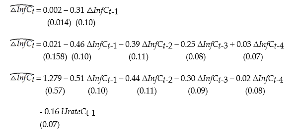 In addition, you have the following information on inflation in Canada during the four quarters of 1999 and the first quarter of 2000:
Inflation and Unemployment in Canada, First Quarter 1999 to First Quarter 2000 Quarter Unemployment Rate Rate of Inflation at an First Lag ( Inf -1) Change in Inflation Annual Rate Inf \Delta Inf 1999:I 7.7 0.8 0.8 0.0 1999: II 7.9 4.3 0.8 3.5 1999: III 7.7 2.9 4.3 -1.4 1999: IV 7.0 1.3 2.9 -1.5 2000:I 6.8 2.1 1.3 0.8 For each of the three models, calculate the predicted inflation rate for the period 2000:I and the forecast error.
(d)Perform a test on whether or not Canadian unemployment rates Granger-cause the Canadian inflation rate.
In addition, you have the following information on inflation in Canada during the four quarters of 1999 and the first quarter of 2000:
Inflation and Unemployment in Canada, First Quarter 1999 to First Quarter 2000 Quarter Unemployment Rate Rate of Inflation at an First Lag ( Inf -1) Change in Inflation Annual Rate Inf \Delta Inf 1999:I 7.7 0.8 0.8 0.0 1999: II 7.9 4.3 0.8 3.5 1999: III 7.7 2.9 4.3 -1.4 1999: IV 7.0 1.3 2.9 -1.5 2000:I 6.8 2.1 1.3 0.8 For each of the three models, calculate the predicted inflation rate for the period 2000:I and the forecast error.
(d)Perform a test on whether or not Canadian unemployment rates Granger-cause the Canadian inflation rate.
(Essay)
5.0/5 (41)
Statistical inference was a concept that was not too difficult to understand when using cross-sectional data. For example, it is obvious that a population mean is not the same as a sample mean (take weight of students at your college/university as an example). With a bit of thought, it also became clear that the sample mean had a distribution. This meant that there was uncertainty regarding the population mean given the sample information, and that you had to consider confidence intervals when making statements about the population mean. The same concept carried over into the two-dimensional analysis of a simple regression: knowing the height-weight relationship for a sample of students, for example, allowed you to make statements about the population height-weight relationship. In other words, it was easy to understand the relationship between a sample and a population in cross-sections. But what about time-series? Why should you be allowed to make statistical inference about some population, given a sample at hand (using quarterly data from 1962-2010, for example)? Write an essay explaining the relationship between a sample and a population when using time series.
(Essay)
4.9/5 (39)
(Requires Appendix material)Define the difference operator Δ = (1 - L)where L is the lag operator, such that LjYt = Yt-j. In general, = (1- Lj)i, where i and j are typically omitted when they take the value of 1. Show the expressions in Y only when applying the difference operator to the following expressions, and give the resulting expression an economic interpretation, assuming that you are working with quarterly data:
(a)Δ4Yt
(b) Yt
(c) Yt
(d) Yt
(Essay)
4.9/5 (33)
The Bayes-Schwarz Information Criterion (BIC)is given by the following formula
(Multiple Choice)
4.9/5 (27)
Filters
- Essay(0)
- Multiple Choice(0)
- Short Answer(0)
- True False(0)
- Matching(0)