Exam 14: Introduction to Time Series Regression and Forecasting
Exam 1: Economic Questions and Data17 Questions
Exam 2: Review of Probability70 Questions
Exam 3: Review of Statistics65 Questions
Exam 4: Linear Regression With One Regressor65 Questions
Exam 5: Regression With a Single Regressor: Hypothesis Tests and Confidence Intervals59 Questions
Exam 6: Linear Regression With Multiple Regressors65 Questions
Exam 7: Hypothesis Tests and Confidence Intervals in Multiple Regression64 Questions
Exam 8: Nonlinear Regression Functions63 Questions
Exam 9: Assessing Studies Based on Multiple Regression65 Questions
Exam 10: Regression With Panel Data50 Questions
Exam 11: Regression With a Binary Dependent Variable50 Questions
Exam 12: Instrumental Variables Regression50 Questions
Exam 13: Experiments and Quasi-Experiments50 Questions
Exam 14: Introduction to Time Series Regression and Forecasting50 Questions
Exam 15: Estimation of Dynamic Causal Effects50 Questions
Exam 16: Additional Topics in Time Series Regression50 Questions
Exam 17: The Theory of Linear Regression With One Regressor49 Questions
Exam 18: The Theory of Multiple Regression50 Questions
Select questions type
Find data for real GDP (Yt)for the United States for the time period 1959:I (first quarter)to 1995:IV. Next generate two growth rates: The (annualized)quarterly growth rate of real GDP
[(lnYt - lnYt-1)× 400] and the annual growth rate of real GDP [(lnYt - lnYt-4)× 100]. Which is more volatile? What is the reason for this? Explain.
(Essay)
5.0/5  (36)
(36)
Consider the standard AR(1)Yt = β0 + β1Yt-1 + ut, where the usual assumptions hold.
(a)Show that yt = β0Yt-1 + ut, where yt is Yt with the mean removed, i.e., yt = Yt - E(Yt). Show that E(Yt)= 0.
(b)Show that the r-period ahead forecast E( +r
)= If 0 < β1 < 1, how does the r-period ahead forecast behave as r becomes large? What is the forecast of for large r?
(c)The median lag is the number of periods it takes a time series with zero mean to halve its current value (in expectation), i.e., the solution r to E( +r
)= 0.5 Show that in the present case this is given by r = -
(Essay)
4.8/5 (27)
Consider the AR(1)model Yt = β0 + β1Yt-1 + ut, < 1..
(a)Find the mean and variance of Yt.
(b)Find the first two autocovariances of Yt.
(c)Find the first two autocorrelations of Yt.
(Essay)
4.8/5 (25)
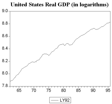
The following two graphs give you a plot of the United States aggregate unemployment rate for the sample period 1962:I to 1999:IV, and the (log)level of real United States GDP for the sample period 1962:I to 1995:IV. You want test for stationarity in both cases. Indicate whether or not you should include a time trend in your Augmented Dickey-Fuller test and why. 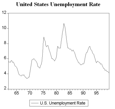
(Essay)
4.8/5 (38)
You have decided to use the Dickey Fuller (DF)test on the United States aggregate unemployment rate (sample period 1962:I - 1995:IV). As a result, you estimate the following AR(1)model t = 0.114 - 0.024 UrateUSt-1, R2 = 0.0118, SER = 0.3417
(0.121)(0.019)
You recall that your textbook mentioned that this form of the AR(1)is convenient because it allows for you to test for the presence of a unit root by using the t- statistic of the slope. Being adventurous, you decide to estimate the original form of the AR(1)instead, which results in the following output t = 0.114 - 0.976 UrateUSt-1, R2 = 0.9510, SER = 0.3417
(0.121)(0.019)
You are surprised to find the constant, the standard errors of the two coefficients, and the SER unchanged, while the regression R2 increased substantially. Explain this increase in the regression R2. Why should you have been able to predict the change in the slope coefficient and the constancy of the standard errors of the two coefficients and the SER?
(Essay)
4.9/5 (40)
You want to determine whether or not the unemployment rate for the United States has a stochastic trend using the Augmented Dickey Fuller Test (ADF). The BIC suggests using 3 lags, while the AIC suggests 4 lags.
(a)Which of the two will you use for your choice of the optimal lag length?
(b)After estimating the appropriate equation, the t-statistic on the lag level unemployment rate is (-2.186)(using a constant, but not a trend). What is your decision regarding the stochastic trend of the unemployment rate series in the United States?
(c)Having worked in the previous exercise with the unemployment rate level, you repeat the exercise using the difference in United States unemployment rates. Write down the appropriate equation to conduct the Augmented Dickey-Fuller test here. The t-statistic on relevant coefficient turns out to be (-4.791). What is your conclusion now?
(Essay)
4.8/5 (37)
(Requires Appendix material)The long-run, stationary state solution of an AD(p,q)model, which can be written as A(L)Yt = ?0 + c(L)Xt-1 + ut, where = 1, and = -?j, cj = ?j, can be found by setting L=1 in the two lag polynomials. Explain. Derive the long-run solution for the estimated ADL(4,4)of the change in the inflation rate on unemployment:
t = 1.32 - .36 ?Inft-1 - 0.34vInft-2 + 0.7?Inft-3 - 0.3?Inft-4
-2.68Unempt-1 + 3.43Unempt-2 - 1.04Unempt-3 + .07Unempt-4
Assume that the inflation rate is constant in the long-run and calculate the resulting unemployment rate. What does the solution represent? Is it reasonable to assume that this long-run solution is constant over the estimation period 1962-1999? If not, how could you detect the instability?
(Essay)
4.9/5 (32)
Consider the following model
Yt = α0 + α1
+ ut
where the superscript "e" indicates expected values. This may represent an example where consumption depended on expected, or "permanent," income. Furthermore, let expected income be formed as follows: = + λ(Xt-1 - ); 0 < λ < 1
This particular type of expectation formation is called the "adaptive expectations hypothesis."
(a)In the above expectation formation hypothesis, expectations are formed at the beginning of the period, say the 1st of January if you had annual data. Give an intuitive explanation for this process.
(b)Transform the adaptive expectation hypothesis in such a way that the right hand side of the equation only contains observable variables, i.e., no expectations.
(c)Show that by substituting the resulting equation from the previous question into the original equation, you get an ADL(0, ∞)type equation. How are the coefficients of the regressors related to each other?
(d)Can you think of a transformation of the ADL(0, ∞)equation into an ADL(1,1)type equation, if you allowed the error term to be (ut - λut-1)?
(Essay)
4.8/5 (36)
You have collected data for real GDP (Y)and have estimated the following function:
ln t = 7.866 + 0.00679×Zeit
(0.007)(0.00008)
t = 1961:I - 2007:IV, R2 = 0.98, SER = 0.036
where Zeit is a deterministic time trend, which takes on the value of 1 during the first quarter of 1961, and is increased by one for each following quarter.
a. Interpret the slope coefficient. Does it make sense?
b. Interpret the regression R2. Are you impressed by its value?
c. Do you think that given the regression R2, you should use the equation to forecast real GDP beyond the sample period?
(Essay)
4.8/5 (32)
(Requires Appendix material): Show that the AR(1)process Yt = a1Yt-1 + et; < 1, can be converted to a MA(∞)process.
(Essay)
4.9/5 (31)
Filters
- Essay(0)
- Multiple Choice(0)
- Short Answer(0)
- True False(0)
- Matching(0)