Exam 17: Regression Models With Dummy Variables

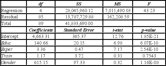
To examine the differences between salaries of male and female middle managers of a large bank, 90 individuals were randomly selected, and two models were created with the following variables considered: Salary = the monthly salary (excluding fringe benefits and bonuses), Educ = the number of years of education, Exper = the number of months of experience, Train = the number of weeks of training, Gender = the gender of an individual; 1 for males, and 0 for females. Excel partial outputs corresponding to these models are available and shown below. 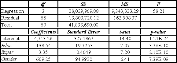Model A: Salary = β₀ + β₁Educ + β₂Exper + β₃Train + β₄Gender + ε Model B: Salary = β₀ + β₁Educ + β₂Exper + β₃Gender + ε The variable Train is deleted from Model A which results in Model B. Which of the following justifies this choice?

Using a ________ we can determine if a particular dummy variable is statistically significant.

According to the Center for Disease Control and Prevention, life expectancy at age 65 in America is about 18.7 years. Medical researchers have argued that while excessive drinking is detrimental to health, drinking a little alcohol every day, especially wine, may be associated with an increase in life expectancy. Others have also linked longevity with income and gender. Data were collected related to the length of life after 65 (Life) were collected including the average income (in $1,000s) (Income), the average number of alcoholic drinks consumed per day (Drinks), and a dummy variable Woman which is 1 when the individual is a woman and 0 otherwise. The following model was created: Life = β₀ + β₁Income + β₂Drinks + β₃Woman + ε. Output corresponding to this model is shown below. Which of the following is the predicted life expectancy for a 65-year-old man with an income of $50,000 and a consumption of three drinks per day?

To encourage performance, loyalty, and continuing education, the human resources department at a large company wants to develop a regression-based compensation model for mid-level managers based on three variables: business unit-profitability in $1,000s (Profit), years with company (Years), and a dummy variable (Grad) which takes on 1 when the individual holds a graduate degree in a relevant field and 0 otherwise. Data have been collected for 36 managers. The sample regression equation is = - 13,264.3 + 14.13Profit + 1,868.53Years + 45,121.94Grad - 0.1539Profit × Grad - 198.34 Years × Grad. Which of the following is the predicted value of Compensation for a manager having 15 years with the company, a graduate degree, and a business-unit profit of $4,800,000?

A researcher wants to examine how the remaining balance on $100,000 loans taken 10 to 20 years ago depends on whether the loan was a prime or subprime loan. He collected a sample of 25 prime loans and 25 subprime loans and recorded the data in the following variables: Balance = the remaining amount of loan to be paid off (in $), Time = the time elapsed from taking the loan, Prime = a dummy variable assuming 1 for prime loans, and 0 for subprime loans. The regression results obtained for the models: Model A: Balance = β₀ + β₁Prime + ε Model B: Balance = β₀ + β₁Time + β₂Prime + β₃Time × Prime + ε Model C: Balance = β₀ + β₁Prime + β₂Time × Prime + ε, Are summarized in the following table. 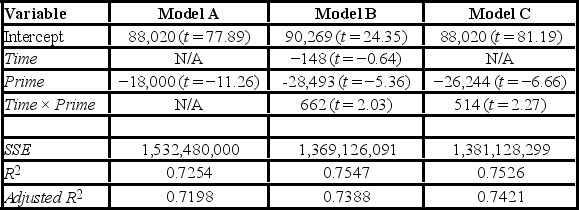Note: The values of relevant test statistics are shown in parentheses below the estimated coefficients. Which of the following three models would you choose to make the predictions of the remaining loan balance?

The method of maximum likelihood estimation (MLE) is used to ________ the parameters of a logit model.

A bank manager is interested in assigning a rating to the holders of credit cards issued by her bank. The rating is based on the probability of defaulting on credit cards and is as follows. To estimate this probability, she decided to use the logit model, P = 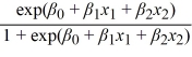, where y = a binary response variable which is 1 if the credit card is in default and 0 otherwise x₁ = the ratio of the credit card balance to the credit card limit (in %) x₂ = the ratio of the total debt to the annual income (in %) The following output is obtained. Note: The p-values of the corresponding tests are shown in parentheses below the estimated coefficients. If only applicants with excellent and good ratings are qualified for a loan, find a linear relation between their balance ratio and their debt ratio that must be satisfied to be qualified.

To examine the differences between salaries of male and female middle managers of a large bank, 90 individuals were randomly selected, and two models were created with the following variables considered: Salary = the monthly salary (excluding fringe benefits and bonuses), Educ = the number of years of education, Exper = the number of months of experience, Train = the number of weeks of training, Gender = the gender of an individual; 1 for males, and 0 for females. Excel partial outputs corresponding to these models are available and shown below. Model A: Salary = β₀ + β₁Educ + β₂Exper + β₃Train + β₄Gender + ε Model B: Salary = β₀ + β₁Educ + β₂Exper + β₃Gender + ε Assuming the same years of education and months of experience, what is the p-value for testing whether the mean salary of males is greater than the mean salary of females using Model B?

Consider the regression equation = b₀ + b₁xd with b₁ > 0 and a dummy variable d. If d changes from 0 to 1, which of the following is true?

A binary choice model is also referred to as a discrete choice model.

A dummy variable is also called an interaction variable.

For the model y = β₀ + β₁x + β₂d₁ + β₃d₂ + ε, which of the following tests is used for testing the joint significance of the dummy variables d₁ and d₂?

A realtor wants to predict and compare the prices of homes in three neighboring locations. She considers the following linear models: Model A: Price = β₀ + β₁ Size + β₂ Age + ε Model B: Price = β₀ + β₁ Size + β₃ Loc1 + β₄ Loc2 + ε Model C: Price = β₀ + β₁ Size + β₂ Age + β₃ Loc1 + β₄ Loc2 + ε where, Price = the price of a home (in $1,000s) Size = the square footage (in sq. feet) Loc1 = a dummy variable taking on 1 for Location 1, and 0 otherwise Loc2 = a dummy variable taking on 1 for Location 2, and 0 otherwise After collecting data on 52 sales and applying regression, her findings were summarized in the following table. Note: The values of relevant test statistics are shown in parentheses below the estimated coefficients. Using Model C, what is the conclusion for testing the joint significance of the two dummy variables at the 1% significance level?

A realtor wants to predict and compare the prices of homes in three neighboring locations. She considers the following linear models: Model A: Price = β₀ + β₁ Size + β₂ Age + ε Model B: Price = β₀ + β₁ Size + β₃ Loc1 + β₄ Loc2 + ε Model C: Price = β₀ + β₁ Size + β₂ Age + β₃ Loc1 + β₄ Loc2 + ε where, Price = the price of a home (in $1,000s) Size = the square footage (in sq. feet) Loc1 = a dummy variable taking on 1 for Location 1, and 0 otherwise Loc2 = a dummy variable taking on 1 for Location 2, and 0 otherwise After collecting data on 52 sales and applying regression, her findings were summarized in the following table. Note: The values of relevant test statistics are shown in parentheses below the estimated coefficients. Using Model B, compute the predicted difference between the price of homes with the same square footage located in Location 2 and Location 3.

The logit model cannot be estimated with standard ________ least squares procedures.

The model y = β₀ + β₁x + β₂d + β₃xd + ε> is an example of a ________.

Like any other university, Seton Hall University uses SAT scores and high school GPAs as primary criteria for admission. Data for 30 students who had recently applied to Seton Hall were collected including admission (1 for admission and 0 otherwise), SAT score, and GPA. Output for the model is shows below. Which of the following is the predicted probability of admission for an individual with a GPA of 3.5 and an SAT score of 1,700?

To examine the differences between salaries of male and female middle managers of a large bank, 90 individuals were randomly selected and the following variables considered: Salary = the monthly salary (excluding fringe benefits and bonuses) Educ = the number of years of education Exper = the number of months of experience Gender = the gender of an individual; 1 for males, and 0 for females The regression results obtained for the models are as follows: Model A: Salary = β₀ + β₁ Educ + β₂ Exper + β₃ Gender + β₄ Exper × Gender + ε, Model B: Salary = β₀ + β₁ Educ + β₂ Exper + ε, are summarized in the following table. Note: The values of relevant test statistics are shown in parentheses below the estimated coefficients. At 1% significance level, what is the conclusion of testing the joint significance of Exper and Exper × Gender in Model A?

For a linear regression model with a dummy variable d and an interaction variable xd, we ________.

The logit model can be estimated with standard ordinary least squares.