Exam 17: Regression Models With Dummy Variables

In the regression equation = b₀ + b₁x + b₂dx with a dummy variable d, when d changes from 0 to 1, the change in the slope of the corresponding lines is given by ________.

Consider the model y = β₀ + β₁x + β₂d + ε, where x is a quantitative variable and d is a dummy variable. When d = 0, the predicted value of y is ________.

The major shortcoming of the general linear probability model y = β₀ + β₁x₁ + β₂x₂ + … + β_kx_k + ε, is that the predicted values of y can be sometimes ________.

To avoid the dummy variable ________, the number of dummy variables should be one less than the number of categories.

To examine the differences between salaries of male and female middle managers of a large bank, 90 individuals were randomly selected, and two models were created with the following variables considered: Salary = the monthly salary (excluding fringe benefits and bonuses), Educ = the number of years of education, Exper = the number of months of experience, Train = the number of weeks of training, Gender = the gender of an individual; 1 for males, and 0 for females. Excel partial outputs corresponding to these models are available and shown below. Model A: Salary = β₀ + β₁Educ + β₂Exper + β₃Train + β₄Gender + ε Model B: Salary = β₀ + β₁Educ + β₂Exper + β₃Gender + ε 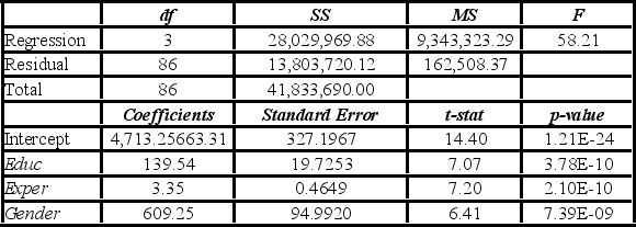Which of the following is the regression equation found by Excel for Model A?

A realtor wants to predict and compare the prices of homes in three neighboring locations. She considers the following linear models: Model A: Price = β₀ + β₁ Size + β₂ Age + ε Model B: Price = β₀ + β₁ Size + β₃ Loc1 + β₄ Loc2 + ε Model C: Price = β₀ + β₁ Size + β₂ Age + β₃ Loc1 + β₄ Loc2 + ε where, Price = the price of a home (in $1,000s) Size = the square footage (in sq. feet) Loc1 = a dummy variable taking on 1 for Location 1, and 0 otherwise Loc2 = a dummy variable taking on 1 for Location 2, and 0 otherwise After collecting data on 52 sales and applying regression, her findings were summarized in the following table. Note: The values of relevant test statistics are shown in parentheses below the estimated coefficients. Using Model B, compute the test statistic for testing the joint significance of the two dummy variables Loc1 and Loc2.

For the linear probability model y = β₀ + β₁x + ε, the predictions made by = b₀ + b₁x can be always interpreted as probabilities.

In the model y = β₀ + β₁x + β₂d + β₃xd + ε, the dummy variable and the interaction variable cause ________.

To examine the differences between salaries of male and female middle managers of a large bank, 90 individuals were randomly selected, and two models were created with the following variables considered: Salary = the monthly salary (excluding fringe benefits and bonuses), Educ = the number of years of education, Exper = the number of months of experience, Train = the number of weeks of training, Gender = the gender of an individual; 1 for males, and 0 for females. Excel partial outputs corresponding to these models are available and shown below. Model A: Salary = β₀ + β₁Educ + β₂Exper + β₃Train + β₄Gender + ε 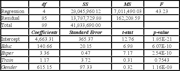Model B: Salary = β₀ + β₁Educ + β₂Exper + β₃Gender + ε 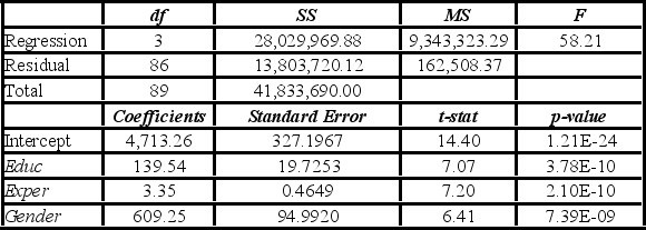Assuming the same years of education and months of experience, what is the null hypothesis for testing whether the mean salary of males is greater than the mean salary of females using Model B?

A medical researcher is interested in assessing the probability of some symptoms of coronary heart disease being present at a given age. For this reason he uses the following data collected on 100 individuals. 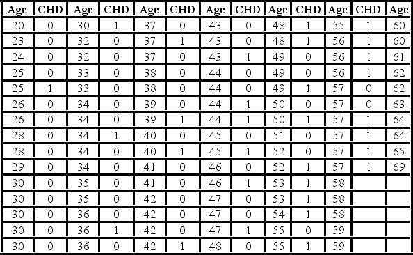The response variable is CHD which is 1 if coronary heart disease is present and 0 otherwise. The following linear probability model and logit model have been estimated: Linear probability: = - 0.53796 + 0.02181Age Logit: = 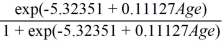Using the logitmodel, find the age of a person for which the estimated chances of having coronary heart disease are 50%?

Which of the following represents a logit regression model?

To encourage performance, loyalty, and continuing education, the human resources department at a large company wants to develop a regression-based compensation model for mid-level managers based on three variables: business unit-profitability in $1,000s (Profit), years with company (Years), and a dummy variable (Grad) which takes on 1 when the individual holds a graduate degree in a relevant field and 0 otherwise. Data have been collected for 36 managers. The sample regression equation is = - 13,264.3 + 14.13Profit + 1,868.53Years + 45,121.94Grad - 0.1539Profit × Grad - 198.34Years × Grad. Which of the following is the difference in the predicted compensations for two managers, one having graduate degree, the other one not, both having 10 years with the company, and having the same business-unit profit of $3,000,000?

A dummy variable is a variable that takes on the values of 0 and 1.

A realtor wants to predict and compare the prices of homes in three neighboring locations. She considers the following linear models: Model A: Price = β₀ + β₁ Size + β₂ Age + ε Model B: Price = β₀ + β₁ Size + β₃ Loc1 + β₄ Loc2 + ε Model C: Price = β₀ + β₁ Size + β₂ Age + β₃ Loc1 + β₄ Loc2 + ε where, Price = the price of a home (in $1,000s) Size = the square footage (in sq. feet) Loc1 = a dummy variable taking on 1 for Location 1, and 0 otherwise Loc2 = a dummy variable taking on 1 for Location 2, and 0 otherwise After collecting data on 52 sales and applying regression, her findings were summarized in the following table. Note: The values of relevant test statistics are shown in parentheses below the estimated coefficients. Using Model C, define the null hypothesis for testing the joint significance of the two dummy variables.

A researcher has developed the following regression equation to predict the prices of luxurious Oceanside condominium units, = 40 + 0.15Size + 50View, where Price = the price of a unit (in $1,000s), Size is the square footage (in sq. feet), and View is a dummy variable taking on 1 for an ocean view unit and 0 for a bay view unit. Which of the following is the predicted price of an ocean view unit with 1,500 square feet?

A researcher wants to examine how the remaining balance on $100,000 loans taken 10 to 20 years ago depends on whether the loan was a prime or subprime loan. He collected a sample of 25 prime loans and 25 subprime loans and recorded the data in the following variables: Balance = the remaining amount of loan to be paid off (in $), Time = the time elapsed from taking the loan, Prime = a dummy variable assuming 1 for prime loans, and 0 for subprime loans. The regression results obtained for the models: Model A: Balance = β₀ + β₁Prime + ε Model B: Balance = β₀ + β₁Time + β₂Prime + β₃Time × Prime + ε Model C: Balance = β₀ + β₁Prime + β₂Time × Prime + ε, Are summarized in the following table. 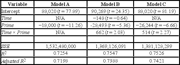Note: The values of relevant test statistics are shown in parentheses below the estimated coefficients. Using Model C, what is the predicted balance on a $100,000 subprime loan taken 15 years ago?

Regression models that use a binary variable as the response variable are called binary choice models.

A dummy variable can be used to create a(n) ________ variable between the dummy variable and a quantitative variable x, which allows the predicted y to differ between the two categories by a varying amount across the values of x.

To examine the differences between salaries of male and female middle managers of a large bank, 90 individuals were randomly selected, and two models were created with the following variables considered: Salary = the monthly salary (excluding fringe benefits and bonuses), Educ = the number of years of education, Exper = the number of months of experience, Train = the number of weeks of training, Gender = the gender of an individual; 1 for males, and 0 for females. Excel partial outputs corresponding to these models are available and shown below. Model A: Salary = β₀ + β₁Educ + β₂Exper + β₃Train + β₄Gender + ε 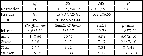Model B: Salary = β₀ + β₁Educ + β₂Exper + β₃Gender + ε For a test of individual significance about gender, what is the conclusion at 5% significance level?

A dummy variable is also referred to as a(n) ________ variable.