Exam 7: Linear Regression
Exam 1: Stats Starts Here33 Questions
Exam 2: Displaying and Describing Categorical Data70 Questions
Exam 3: Displaying and Summarizing Quantitative Data148 Questions
Exam 4: Understanding and Comparing Distributions46 Questions
Exam 5: The Standard Deviation As a Ruler and the Normal Model111 Questions
Exam 6: Scatterplots, association, and Correlation78 Questions
Exam 7: Linear Regression71 Questions
Exam 8: Regression Wisdom32 Questions
Exam 9: Understanding Randomness26 Questions
Exam 10: Sample Surveys64 Questions
Exam 11: Experiments and Observational Studies80 Questions
Exam 12: From Randomness to Probability69 Questions
Exam 13: Probability Rules95 Questions
Exam 14: Random Variables215 Questions
Exam 15: Sampling Distribution Models51 Questions
Exam 16: Confidence Intervals for Proportions71 Questions
Exam 17: Testing Hypotheses About Proportions44 Questions
Exam 18: More About Tests67 Questions
Exam 19: Comparing Two Proportions53 Questions
Exam 20: Inferences About Means123 Questions
Exam 21: Comparing Means50 Questions
Exam 22: Paired Samples and Blocks35 Questions
Exam 23: Comparing Counts76 Questions
Exam 24: Inferences for Regression57 Questions
Exam 25: Analysis of Variance39 Questions
Exam 26: Multifactor Analysis of Variance22 Questions
Exam 27: Multiple Regression22 Questions
Exam 28: Multiple Regression Wisdom21 Questions
Exam 29: Rank-Based Nonparametric Tests29 Questions
Exam 30: The Bootstrap27 Questions
Select questions type
The relationship between two quantities x and y is examined.The relationship appears to be fairly linear.A linear model is considered,and the regression analysis is as follows: Dependent variable: y
R-squared = 87.9%
VARIABLE COEFFICIENT
Intercept 37.74
X -9.97
What does the slope say about the relationship between x and y?
(Multiple Choice)
4.8/5  (42)
(42)
Ten Jeep Cherokee classified ads were selected.The age and prices of several used Ford Escorts are given in the table. Age (years) Price 1 \ 19,000 1 \ 18,500 2 \ 16,000 3 \ 13,000 3 \ 12,600 4 \ 10,000 4 \ 9000 5 \ 6000 6 \ 4000 6 \ 2900
(Multiple Choice)
4.9/5 (33)
A random sample of records of electricity usage of homes in the month of July gives the amount of electricity used and size (in square feet)of 135 homes.A regression was done to predict the amount of electricity used (in kilowatt-hours)from size.Suppose the linear model is appropriate.The model is size.How much electricity would you predict would be used in a house that is 2372 square feet?
(Multiple Choice)
4.8/5 (36)
The relationship between two quantities X and Y is examined,and the association is shown in the scatterplot below. 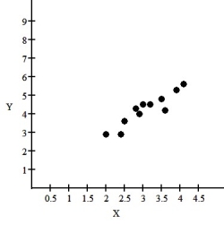 If a linear model is considered,the regression analysis is as follows: Dependent variable: Y
R-squared = 84.7%
VARIABLE COEFFICIENT
Intercept 1.2305
X .4443
What does the slope say about this relationship?
If a linear model is considered,the regression analysis is as follows: Dependent variable: Y
R-squared = 84.7%
VARIABLE COEFFICIENT
Intercept 1.2305
X .4443
What does the slope say about this relationship?
(Multiple Choice)
4.8/5 (37)
The relationship between the cost of a taxi ride (y)and the length of the ride (x)is analyzed.The mean length was 4.6 km with a standard deviation of 1.1.The mean cost was $8.70 with a standard deviation of 2.0.The correlation between the cost and the length was 0.81.
(Multiple Choice)
4.9/5 (28)
Using advertised prices for used Ford Escorts a linear model for the relationship between a car's age and its price is found.The regression has an = 85.8%.Why doesn't the model explain 100% of the variation in the price of an Escort?
(Multiple Choice)
4.9/5 (40)
The relationship between the number of games won by an NHL team and the average attendance at their home games is analyzed.A regression to predict the average attendance from the number of games won has an = 30.4%.The residuals plot indicated that a linear model is appropriate.Write a sentence summarizing what says about this regression.
(Multiple Choice)
4.8/5 (37)
A forester would like to know how big a maple tree might be at age 50 years.She gathers data from some trees that have been cut down,and plots the diameters (in inches)of the trees against their ages (in years).She re-expresses the data,using the logarithm of age to try to predict the diameter of the tree.Here are the regression analysis and the residuals plot.Explain why you think this is an appropriate model. Dependent variable is: Diam
Rsquared
Constant
Log(Age) 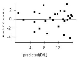
(Essay)
4.8/5 (38)
The relationship between the number of games won by an NHL team and the average attendance at their home games is analyzed.A regression to predict the average attendance from the number of games won has an = 31.4%.The residuals plot indicated that a linear model is appropriate.What is the correlation between the average attendance and the number of games won.
(Multiple Choice)
4.7/5 (39)
The relationship between the selling price (in dollars)of used Ford Escorts and their age (in years)is analyzed.A regression analysis to predict the price from the age gives the model age.Predict the price of an Escort that is 8 years old.
(Multiple Choice)
4.9/5 (33)
Doctors studying how the human body assimilates medication inject some patients with penicillin,and then monitor the concentration of the drug (in units/cc)in the patients' blood for seven hours.The researchers try model,using the re-expression log(Concentration).Examine the regression analysis and the residuals plot below.Explain why you think this model is appropriate. Dependent variable is: LogCnn
No Selector
R squared R squared (adjusted)
with degrees of freedom
Source Sum of Squares df Mean Square F-ratio Regression 4.11395 1 4.11395 2022 Residual 0.083412 41 0.002034
Variable Coefficient s.e. of Coeff t.ratio prob Constant 1.80184 0.0168 107 0.0001 Time -0.172672 0.0038 -45.0 S.0.0001 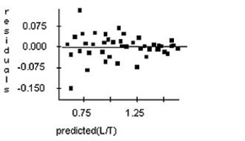
(Essay)
4.7/5 (33)
A random sample of records of electricity usage of homes gives the amount of electricity used in July and size (in square feet)of 135 homes.A regression to predict the amount of electricity used (in kilowatt-hours)from size was completed.What are the variables and units in this regression?
(Multiple Choice)
4.8/5 (49)
A random sample of 150 yachts sold in Canada last year was taken.A regression to predict the price (in thousands of dollars)from length (in metres)has an What would you predict about the price of the yacht whose length was two standard deviations below the mean?
(Multiple Choice)
4.9/5 (37)
Two different tests are designed to measure employee productivity and dexterity.Several employees are randomly selected and tested with these results. Dexterity
Productivity 23 25 28 21 21 25 26 30 34 36 49 53 59 42 47 53 55 63 67 75
(Multiple Choice)
4.8/5 (35)
Ten students in a tutor program at Carleton University were randomly selected.Their grade point averages (GPAs)when they entered the program were less than 9.5.The following data were obtained regarding their GPAs on entering the program versus their current GPAs. Entering GPA (E) Current GPA (C) 9.5 9.6 8.8 9.1 9.3 9.5 8.6 8.6 8.5 9.0 9.0 9.4 9.1 9.2 9.4 9.7 8.9 9.3 9.1 9.3
(Multiple Choice)
4.8/5 (40)
Filters
- Essay(0)
- Multiple Choice(0)
- Short Answer(0)
- True False(0)
- Matching(0)