Exam 10: Inference for Regression

There is an old saying in golf: "You drive for show and you putt for dough." The point is that good putting is more important than long driving for shooting low scores and hence winning money.To see if this is the case,data on the top 69 money winners on the PGA tour in 1993 are examined.The average number of putts per hole for each player is used to predict the total winnings (in thousands of dollars)using the simple linear regression model (1993 winnings)_i = ₀ + ₁(average number of putts per hole)_i + _i, Where the deviations _i are assumed to be independent and Normally distributed with a mean of 0 and a standard deviation of .This model was fit to the data using the method of least squares.The following results were obtained from statistical software. 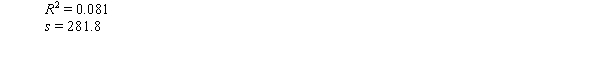Which of the following conclusions seems most justified?

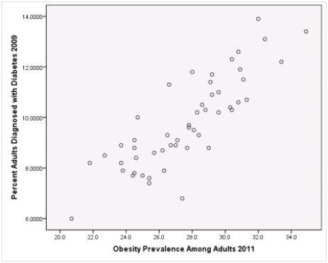
As in most professional sports,statistics are collected in the National Hockey League.In the 2006-2007 season,teams played 82 games.A team was awarded 2 points for a win and 1 point if the game was tied at the end of regulation time but then lost in overtime.For each of the 30 teams,data on the number of goals scored per game (Goals/G)and the percentage of the 164 possible points they won (Win%)during the season were collected.The following graph shows the plotted points for the variables Win% and Goals/G and the simple linear regression line fitted using least squares. From the computer output for the least-squares fit,the estimated equation was found to be , = 0.398,and = 60.29.Also,it was determined from the output that = 12.800 and = 4.418. If a test of hypothesis were conducted of H₀: = 0 against H_a:  0,what would be the value of the test statistic?

A random sample of 79 companies from the Forbes 500 list (which actually consists of nearly 800 companies)was selected,and the relationship between sales (in hundreds of thousands of dollars)and profits (in hundreds of thousands of dollars)was investigated by regression.The following results were obtained from statistical software. Suppose the researchers conducting this study wish to estimate the profits (in hundreds of thousands of dollars)for companies that had sales (in hundreds of thousands of dollars)of 500.The following results were obtained from statistical software. 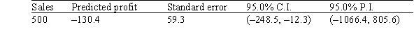If the researchers wish to estimate the profits for a particular company that had sales of 500,what would be a 95% prediction interval for the profits?

Suppose we are given the following information: Sample size,n,= 100 Standard error of slope of the regression line, = 2 = 100 + 4x What is the critical value,t^*,that is used to compute an 80% confidence interval for ₁? (Note: Use software to compute the exact value. )

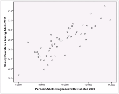
A recent study was done to assess factors that put Hispanic populations more at risk for obesity and related chronic diseases,such as diabetes and heart disease,than non-Hispanic populations.Data were collected on several factors,such as the crude morality rate of Hispanics,obesity prevalence,percent of adults diagnosed with diabetes,and median income at the state level.Pearson's Correlations were used to examine the strength of the relationship between obesity and the other variables,as a way of observing which characteristics were associated with high prevalence of obesity.In addition,a simple linear regression was used to model the relationship between diabetes and obesity.The results from SPSS are shown below. What is the value of the F statistic to test the null hypothesis that versus the alternative hypothesis that ?

A random sample of 79 companies from the Forbes 500 list (which actually consists of nearly 800 companies)was selected,and the relationship between sales (in hundreds of thousands of dollars)and profits (in hundreds of thousands of dollars)was investigated by regression.The following results were obtained from statistical software. Suppose the researchers conducting the study wish to test the hypotheses H₀: ₁ = 0 versus H_a: ₁> 0.What do we know about the P-value of this test?

Which of the following statements about the simple linear regression model and its least squares fit is/are FALSE?

A recent study was done to assess factors that put Hispanic populations more at risk for obesity and related chronic diseases,such as diabetes and heart disease,than non-Hispanic populations.Data were collected on several factors,such as the crude morality rate of Hispanics,obesity prevalence,percent of adults diagnosed with diabetes,and median income at the state level.Pearson's Correlations were used to examine the strength of the relationship between obesity and the other variables,as a way of observing which characteristics were associated with high prevalence of obesity.In addition,a simple linear regression was used to model the relationship between diabetes and obesity.The results from SPSS are shown below. 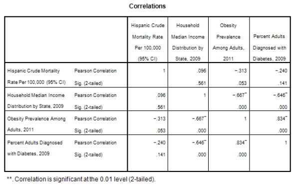What is the P-value to test that the population correlation is zero verses the alternative that the population correlation is greater than zero?

Suppose we are given the following information: Sample size,n,= 100 Standard error of slope of the regression line, = 2 = 100 + 4x Is there a statistically significant linear relationship between the response and explanatory variable when the significance level,,is .01?

Suppose we are given the following information: Sample size,n,= 100 Standard error of slope of the regression line, = 2 = 100 + 4x Suppose an observed response value is 150 when x = 5.What is the value of the residual?

Suppose we are given the following information: Sample size,n,= 100 Standard error of slope of the regression line, = 2 = 100 + 4x What is an 80% confidence interval for ₁?

There is an old saying in golf: "You drive for show and you putt for dough." The point is that good putting is more important than long driving for shooting low scores and hence winning money.To see if this is the case,data on the top 69 money winners on the PGA tour in 1993 are examined.The average number of putts per hole for each player is used to predict the total winnings (in thousands of dollars)using the simple linear regression model (1993 winnings)_i = ₀ + ₁(average number of putts per hole)_i + _i, Where the deviations _i are assumed to be independent and Normally distributed with a mean of 0 and a standard deviation of .This model was fit to the data using the method of least squares.The following results were obtained from statistical software. The quantity s = 281.8 is an estimate of the standard deviation  of the deviations in the simple linear regression model.What are the degrees of freedom for this estimate?

Suppose we are given the following information: Sample size,n,= 100 Standard error of slope of the regression line, = 2 = 100 + 4x Would a 95% confidence interval for ₁ be larger,smaller,or the same as an 80% confidence interval for ₁?

A study was conducted to monitor the emissions of a noxious substance from a chemical plant and the concentration of the chemical at a location in close proximity to the plant at various times throughout the year.A total of 14 measurements were made.Computer output for the simple linear regression least-squares fit is provided.(Some entries have been omitted and replaced with **. ) What is the 95% confidence interval estimate for ?

The statistical model for simple linear regression is written as 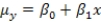,where represents the mean of a Normally distributed response variable and x represents the explanatory variable.The parameters and are estimated,giving the linear regression model defined by ,with standard deviation  = 5. What is the slope of the regression line?

Suppose you are testing the null hypothesis that the slope of the regression line is zero versus the alternative hypothesis that the slope is different than zero.Would a very small P-value indicate a strong relationship between the explanatory variable and the response variable?

As in most professional sports,statistics are collected in the National Hockey League.In the 2006-2007 season,teams played 82 games.A team was awarded 2 points for a win and 1 point if the game was tied at the end of regulation time but then lost in overtime.For each of the 30 teams,data on the number of goals scored per game (Goals/G)and the percentage of the 164 possible points they won (Win%)during the season were collected.The following graph shows the plotted points for the variables Win% and Goals/G and the simple linear regression line fitted using least squares. 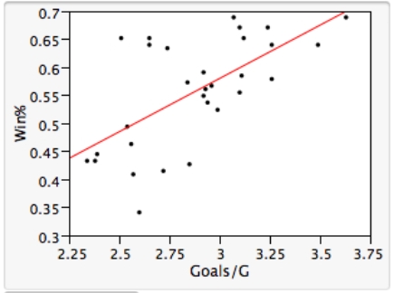From the computer output for the least-squares fit,the estimated equation was found to be = 0.398,and = 60.29.Also,it was determined from the output that = 12.800 and = 4.418.For the 2006-2007 season,teams scored an average of = 2.88 goals per game.For the population of teams that score 2.5 goals per game,the standard error of the estimated mean Win% is = 2.197.What is the estimated mean Win% for the population of teams that score 2.5 goals per game?

A recent study was done to assess factors that put Hispanic populations more at risk for obesity and related chronic diseases,such as diabetes and heart disease,than non-Hispanic populations.Data were collected on several factors,such as the crude morality rate of Hispanics,obesity prevalence,percent of adults diagnosed with diabetes,and median income at the state level.Pearson's Correlations were used to examine the strength of the relationship between obesity and the other variables,as a way of observing which characteristics were associated with high prevalence of obesity.In addition,a simple linear regression was used to model the relationship between diabetes and obesity.The results from SPSS are shown below. 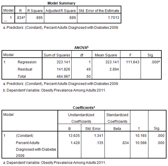What is the standard error of the intercept b₀ of the least-squares regression line for predicting obesity rates from diabetes rates?

A study was conducted to monitor the emissions of a noxious substance from a chemical plant and the concentration of the chemical at a location in close proximity to the plant at various times throughout the year.A total of 14 measurements were made.Computer output for the simple linear regression least-squares fit is provided.(Some entries have been omitted and replaced with **. ) 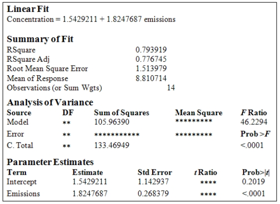What is the estimate of ?

Suppose we are given the following information: Sample size,n,= 100 Standard error of slope of the regression line, = 2 = 100 + 4x What is the test statistic to test the null hypothesis that the slope is zero versus the alternative hypothesis that the slope is not zero?