Exam 10: Inference for Regression

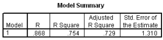
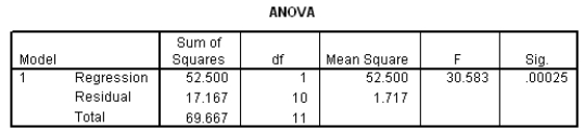
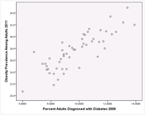
A recent study was done to assess factors that put Hispanic populations more at risk for obesity and related chronic diseases,such as diabetes and heart disease,than non-Hispanic populations.Data were collected on several factors,such as the crude morality rate of Hispanics,obesity prevalence,percent of adults diagnosed with diabetes,and median income at the state level.Pearson's Correlations were used to examine the strength of the relationship between obesity and the other variables,as a way of observing which characteristics were associated with high prevalence of obesity.In addition,a simple linear regression was used to model the relationship between diabetes and obesity.The results from SPSS are shown below. 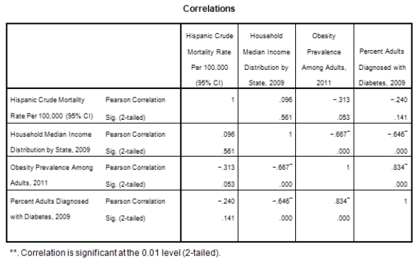What is the standard error of the slope b₁ of the least-squares regression line for predicting obesity rates from diabetes rates?

The statistical model for simple linear regression is written as 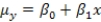,where represents the mean of a Normally distributed response variable and x represents the explanatory variable.The parameters and are estimated,giving the linear regression model defined by ,with standard deviation  = 5. What is the subpopulation mean when x = 20?

A study was conducted to monitor the emissions of a noxious substance from a chemical plant and the concentration of the chemical at a location in close proximity to the plant at various times throughout the year.A total of 14 measurements were made.Computer output for the simple linear regression least-squares fit is provided.(Some entries have been omitted and replaced with **. ) 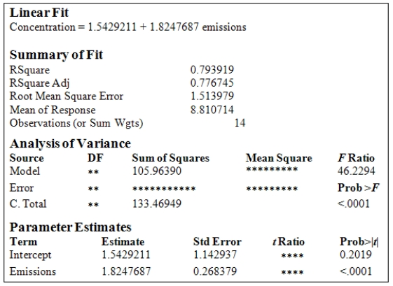What is the test statistic and its value to test H₀: = 0 against H_a:  0?

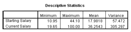
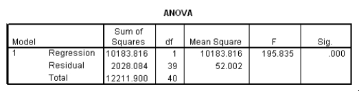
The data referred to in this question were collected on 41 employees of a large company.The company is trying to predict the current salary of its employees from their starting salary (both expressed in thousands of dollars).The SPPS regression output is given below as well as some summary measures: Suppose we wish to test the hypotheses H₀: ₁ = 2 versus H_a: ₁  2.Together with an insignificant constant in this model,this would imply that the employees currently earn about twice as much as their starting salary.At the 5% significance level,would we reject the null hypothesis?

A random sample of 79 companies from the Forbes 500 list (which actually consists of nearly 800 companies)was selected,and the relationship between sales (in hundreds of thousands of dollars)and profits (in hundreds of thousands of dollars)was investigated by regression.The following results were obtained from statistical software. 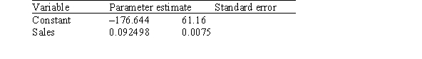The following (partial)ANOVA table was obtained from statistical software. 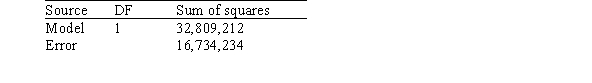What is the value of the SST,the total sum of squares?

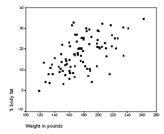
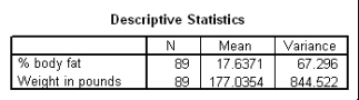
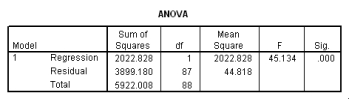
The following scatter plot and SPSS output represent data collected on 89 middle-aged people.The relationship between body weight and percent body fat is to be studied. 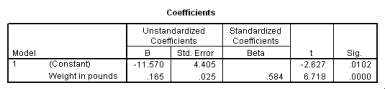Let  be the population correlation between body fat and body weight.What is the value of the t statistic for testing the hypotheses H₀:  = 0 versus H_a:   0?

An interval used to predict a future value is called a ______.

Do heavier cars use more gasoline? To answer this question,a researcher randomly selected 15 cars.He collected their weight (in hundreds of pounds)and the mileage (MPG)for each car.From a scatter plot made with the data,a linear model seemed appropriate.The following output was obtained from SPSS: 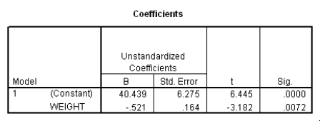To test if there is a significant straight-line relationship between the weight and the mileage of a car,we can perform a t test.What is the value of the t statistic for this test?

The data referred to in this question were collected on 41 employees of a large company.The company is trying to predict the current salary of its employees from their starting salary (both expressed in thousands of dollars).The SPSS regression output is given below as well as some summary measures: How would a 90% confidence interval for the average current salary for all employees who started with a salary of $15,300 compare to a 90% confidence interval for the current salary of an individual with a starting salary of $15,300?

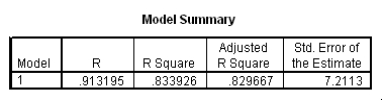
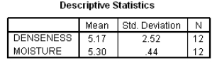
The moisture in a wet mix of cement was considered to have an effect on the denseness of the finished product.The moisture of the mix was controlled at various levels,and the denseness of the finished product was measured.The data were entered into SPSS,and the following output was generated. 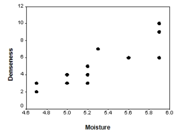What is the equation of the least-squares regression line?

The moisture in a wet mix of cement was considered to have an effect on the denseness of the finished product.The moisture of the mix was controlled at various levels,and the denseness of the finished product was measured.The data were entered into SPSS,and the following output was generated. 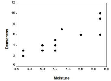What is an approximate 99% confidence interval for the mean denseness of the finished product when the moisture level in the cement mix is 5.5?

What is an approximate 95% confidence interval for the slope ₁?

A recent study was done to assess factors that put Hispanic populations more at risk for obesity and related chronic diseases,such as diabetes and heart disease,than non-Hispanic populations.Data were collected on several factors,such as the crude morality rate of Hispanics,obesity prevalence,percent of adults diagnosed with diabetes,and median income at the state level.Pearson's Correlations were used to examine the strength of the relationship between obesity and the other variables,as a way of observing which characteristics were associated with high prevalence of obesity.In addition,a simple linear regression was used to model the relationship between diabetes and obesity.The results from SPSS are shown below. 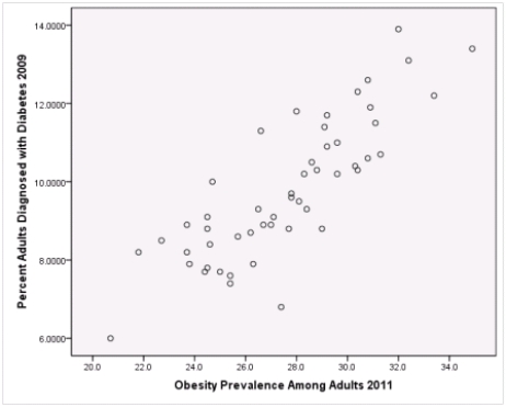What is the sample correlation between obesity prevalence and percent adults diagnosed with diabetes?

Do heavier cars use more gasoline? To answer this question,a researcher randomly selected 15 cars.He collected their weight (in hundreds of pounds)and the mileage (MPG)for each car.From a scatter plot made with the data,a linear model seemed appropriate.The following output was obtained from SPSS: 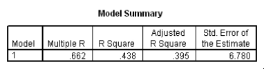What is a 95% confidence interval for the slope ₁?

As in most professional sports,statistics are collected in the National Hockey League.In the 2006-2007 season,teams played 82 games.A team was awarded 2 points for a win and 1 point if the game was tied at the end of regulation time but then lost in overtime.For each of the 30 teams,data on the number of goals scored per game (Goals/G)and the percentage of the 164 possible points they won (Win%)during the season were collected.The following graph shows the plotted points for the variables Win% and Goals/G and the simple linear regression line fitted using least squares. 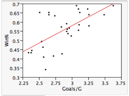From the computer output for the least-squares fit,the estimated equation was found to be , = 0.398,and = 60.29.Also,it was determined from the output that = 12.800 and = 4.418. A plot of the residuals from the least-squares fit against the Goals/G variable is shown below. 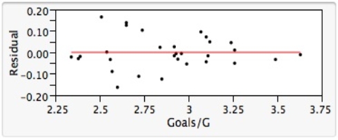What statements about residuals and/or about this residual plot is/are FALSE?

The moisture in a wet mix of cement was considered to have an effect on the denseness of the finished product.The moisture of the mix was controlled at various levels,and the denseness of the finished product was measured.The data were entered into SPSS,and the following output was generated. 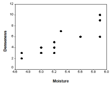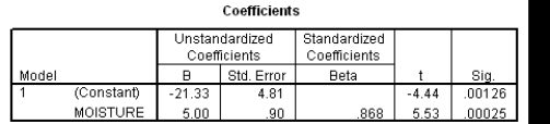Suppose we wish to test if denseness increases with the moisture in the cement mix: H₀: ₁ = 0 versus H_a: ₁> 0.Do we reject the null hypothesis at the 1% significance level?Include the value of the t statistic and the corresponding P-value in your answer.

Which of the following statements about simple linear regression is/are FALSE?

There is an old saying in golf: "You drive for show and you putt for dough." The point is that good putting is more important than long driving for shooting low scores and hence winning money.To see if this is the case,data on the top 69 money winners on the PGA tour in 1993 are examined.The average number of putts per hole for each player is used to predict the total winnings (in thousands of dollars)using the simple linear regression model (1993 winnings)_i = ₀ + ₁(average number of putts per hole)_i + _i, Where the deviations _i are assumed to be independent and Normally distributed with a mean of 0 and a standard deviation of .This model was fit to the data using the method of least squares.The following results were obtained from statistical software. 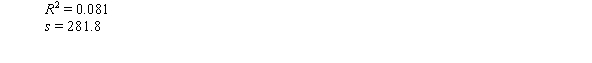Suppose the researchers conducting this study wish to test the hypotheses H₀: ₁ = 0 versus H_a: ₁< 0.What is the value of the t statistic for this test?

The statistical model for simple linear regression is written as ,where represents the mean of a Normally distributed response variable and x represents the explanatory variable.The parameters and are estimated,giving the linear regression model defined by 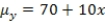,with standard deviation  = 5. What is the distribution of the test statistic used to test the null hypothesis against the alternative hypothesis ? (Note: Assume n is the sample size. )

A recent study was done to assess factors that put Hispanic populations more at risk for obesity and related chronic diseases,such as diabetes and heart disease,than non-Hispanic populations.Data were collected on several factors,such as the crude morality rate of Hispanics,obesity prevalence,percent of adults diagnosed with diabetes,and median income at the state level.Pearson's Correlations were used to examine the strength of the relationship between obesity and the other variables,as a way of observing which characteristics were associated with high prevalence of obesity.In addition,a simple linear regression was used to model the relationship between diabetes and obesity.The results from SPSS are shown below. 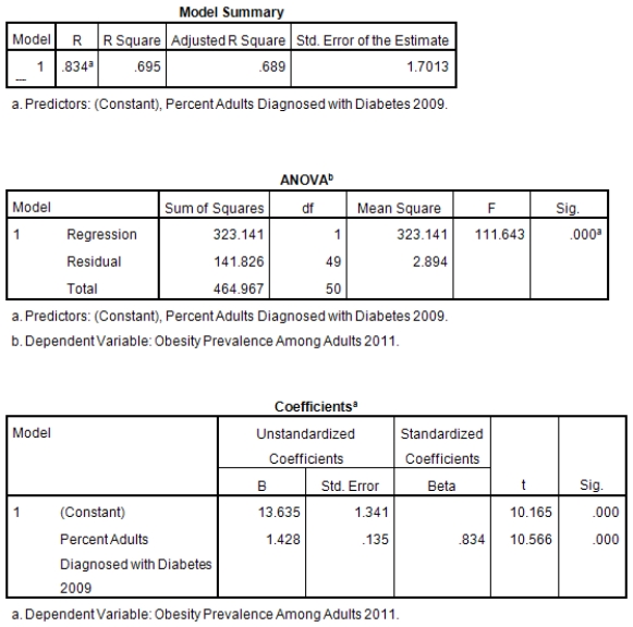What is the sample size?