Exam 19: Multiple Regression

An actuary wanted to develop a model to predict how long individuals will live. After consulting a number of physicians, she collected the age at death (y), the average number of hours of exercise per week ( $x _ { 1 }$ ), the cholesterol level ( $x _ { 2 }$ ), and the number of points by which the individual's blood pressure exceeded the recommended value ( $x _ { 3 }$ ). A random sample of 40 individuals was selected. The computer output of the multiple regression model is shown below: THE REGRESSION EQUATION IS $y=$ $55.8 + 1.79 x _ { 1 } - 0.021 x _ { 2 } - 0.016 x _ { 3 }$ Predictor Coef StDev Constant 55.8 11.8 4.729 1.79 0.44 4.068 -0.021 0.011 -1.909 -0.016 0.014 -1.143 S = 9.47 R-Sq = 22.5%. ANALYSIS OF VARIANCE Source of Variation df SS MS F Regression 3 936 312 3.477 Error 36 3230 89.722 Total 39 4166 Is there enough evidence at the 1% significance level to infer that the average number of hours of exercise per week and the age at death are linearly related?

Given the following statistics of a multiple regression model, can we conclude at the 5% significance level that $x _ { 1 }$ and y are linearly related? n = 42 k = 6 $b _ { 1 } =$ -5.30 $s _ { b _ { 1 } } =$ 1.5

A multiple regression analysis that includes 20 data points and 4 independent variables results in total variation in y = SSY = 200 and SSR = 160. The multiple standard error of estimate will be:

Consider the following statistics of a multiple regression model: n = 30 k = 4 SS_y = 1500 SSE = 260. a. Determine the standard error of estimate. b. Determine the multiple coefficient of determination. c. Determine the F-statistic.

For a set of 30 data points, Excel has found the estimated multiple regression equation to be $\hat{y}$ = -8.61 + 22x₁ + 7x₂ + 28x₃, and has listed the t statistic for testing the significance of each regression coefficient. Using the 5% significance level for testing whether $\beta$ ₃ = 0, the critical region will be that the absolute value of the t statistic for $\beta$ ₃ is greater than or equal to:

Test the hypotheses: $H _ { 0 } :$ There is no first-order autocorrelation $H _ { 1 } :$ There is positive first-order autocorrelation, given that: the Durbin-Watson statistic d = 0.686, n = 16, k = 1 and $\alpha =$ 0.05.

Pop-up coffee vendors have been popular in the city of Adelaide in 2013. A vendor is interested in knowing how temperature (in degrees Celsius) and number of different pastries and biscuits offered to customers impacts daily hot coffee sales revenue (in $00's). A random sample of 6 days was taken, with the daily hot coffee sales revenue and the corresponding temperature and number of different pastries and biscuits offered on that day, noted. Describe the following scatterplots. 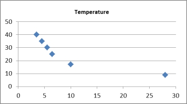Scatterplot of Daily hot coffee sales revenue vs Temperature 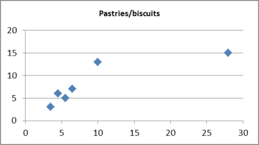Scatterplot of Daily hot coffee sales revenue Pastries/biscuits 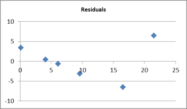Residual scatterplot of Daily hot coffee sales revenue vs fitted values

A multiple regression the coefficient of determination is 0.81. The percentage of the variation in $y$ that is explained by the regression equation is 81%.

Test the hypotheses: $H _ { 0 } :$ There is no first-order autocorrelation $H _ { 1 } :$ There is first-order autocorrelation, given that the Durbin-Watson statistic d = 1.89, n = 28, k = 3 and $\alpha =$ 0.05.

A statistician wanted to determine whether the demographic variables of age, education and income influence the number of hours of television watched per week. A random sample of 25 adults was selected to estimate the multiple regression model $y = \beta _ { 0 } + \beta _ { 1 } x _ { 1 } + \beta _ { 2 } x _ { 2 } + \beta _ { 3 } x _ { 3 } + \varepsilon$ . Where: y = number of hours of television watched last week. $x _ { 1 }$ = age. $x _ { 2 }$ = number of years of education. $x _ { 3 }$ = income (in $1000s). The computer output is shown below. THE REGRESSION EQUATION IS $y =$ $22.3 + 0.41 x _ { 1 } - 0.29 x _ { 2 } - 0.12 x _ { 3 }$ Predictor Coef StDev Constant 22.3 10.7 2.084 0.41 0.19 2.158 -0.29 0.13 -2.231 -0.12 0.03 -4.00 S = 4.51 R-Sq = 34.8%. ANALYSIS OF VARIANCE Source of Variation df SS MS F Regression 3 227 75.667 3.730 Error 21 426 20.286 Total 24 653 What is the coefficient of determination? What does this statistic tell you?

In multiple regression, the standard error of estimate is defined by $S _ { \varepsilon } = \sqrt { SS E / ( n - k ) }$ , where n is the sample size and k is the number of independent variables.

Excel and Minitab both provide the p-value for testing each coefficient in the multiple regression model. In the case of $b _ { 2 }$ , this represents the probability that:

A multiple regression analysis that includes 4 independent variables results in a sum of squares for regression of 1200 and a sum of squares for error of 800. The multiple coefficient of determination will be:

Given the multiple linear regression equation, ŷ = b₀ + b₁x₁ + b₂x₂, the value of b₂ is the estimated average increase in y for a one unit increase in x₂, whilst holding x₁ constant.

In a multiple regression, a large value of the test statistic F indicates that most of the variation in y is explained by the regression equation, and that the model is useful; while a small value of F indicates that most of the variation in y is unexplained by the regression equation, and that the model is useless.

In multiple regression, the problem of multicollinearity affects the t-tests of the individual coefficients as well as the F-test in the analysis of variance for regression, since the F-test combines these t-tests into a single test.

For a multiple regression model with n = 35 and k = 4, the following statistics are given: SS_y = 500 and SSE = 100. The coefficient of determination is:

A statistician estimated the multiple regression model $y = \beta _ { 0 } + \beta _ { 1 } x _ { 1 } + \beta _ { 2 } x _ { 2 } + \varepsilon$ , with 45 observations. The computer output is shown below. However, because of a printer malfunction, some of the results are not shown. These are indicated by the boldface letters a to l. Fill in the missing results (up to three decimal places). Predictor Coef StDev T Constant 6.404 0.007 -0.025 0.383 0.072 c S = d R-Sq = e. ANALYSIS OF VARIANCE Source of Variation SS MS F Regression f i j l Error 11.884 Total h 26.887

If none of the data points for a multiple regression model with two independent variables were on the regression plane, then the multiple coefficient of determination would be:

In testing the validity of a multiple regression model in which there are four independent variables, the null hypothesis is: