Which of the following statistics and procedures can be used to determine whether a linear model should be employed? $\begin{array}{|l|l|} \hline A&\text {The standard error of estimate }\\ \hline B&\text {The coefficient of determination. }\\ \hline C&\text {The \( t $-test of the slope. }\\ \hline D&\text { All of these choices are correct.}\\ \hline \end{array}\)

The answer of Which of the following statistics and procedures...

A financier whose specialty is investing in movie productions has observed that, in general, movies with 'big-name' stars seem to generate more revenue than those movies whose stars are less well known. To examine his belief, he records the gross revenue and the payment (in $ million) given to the two highest-paid performers in the movie for 10 recently released movies. \[\begin{array} { | c | c | c | } \hline \text { Movie } & \begin{array} { c } \text { Cost of two highest- } \\ \text { paid performers } ( \$ \mathrm {~m} ) \end{array} & \begin{array} { c } \text { Gross revenue } \\ ( \$ \mathrm {~m} ) \end{array} \\ \hline 1 & 5.3 & 48 \\ \hline 2 & 7.2 & 65 \\ \hline 3 & 1.3 & 18 \\ \hline 4 & 1.8 & 20 \\ \hline 5 & 3.5 & 31 \\ \hline 6 & 2.6 & 26 \\ \hline 7 & 8.0 & 73 \\ \hline 8 & 2.4 & 23 \\ \hline 9 & 4.5 & 39 \\ \hline 10 & 6.7 & 58 \\ \hline \end{array}\] Conduct a test of the population coefficient of correlation to determine at the 5% significance level whether a linear relationship exists between payment to the two highest-paid performers and gross revenue.

@#IMG-DLM& @#IMG-DLM& Rejection region: | t | > @#IMG-DLM& 2

The regression line Estimated y = 3 + 2x has been fitted to the data points (4,8), (2,5), and (1,2). The sum of the squared residuals will be: $\begin{array}{|l|l|} \hline\text { A. } & 7 . \\ \hline \text { B. } & 15 \\ \hline \text { C. } & 8 . \\ \hline \text { D. } & 22 . \\ \hline \end{array}$

The answer of The regression line Estimated y = 3...

The quality of oil is measured in API gravity degrees - the higher the degrees API, the higher the quality. The table shown below is produced by an expert in the field, who believes that there is a relationship between quality and price per barrel. \[\begin{array} { | c | c | } \hline \text { Oil degrees API } & \text { Price per barrel (in } \$ \text { ) } \\ \hline 27.0 & 12.02 \\ \hline 28.5 & 12.04 \\ \hline 30.8 & 12.32 \\ \hline 31.3 & 12.27 \\ \hline 31.9 & 12.49 \\ \hline 34.5 & 12.70 \\ \hline 34.0 & 12.80 \\ \hline 34.7 & 13.00 \\ \hline 37.0 & 13.00 \\ \hline 41.0 & 13.17 \\ \hline 41.0 & 13.19 \\ \hline 38.8 & 13.22 \\ \hline 39.3 & 13.27 \\ \hline \end{array}\] A partial Minitab output follows. Descriptive Statistics \[\begin{array} { | l | r | r | r | r | } \hline \text { Variable } & \mathrm { N } & \text { Mean } & \text { StDev } & \text { SE Mean } \\ \hline \text { Degrees } & 13 & 34.60 & 4.613 & 1.280 \\ \hline \text { Frice } & 13 & 12.730 & 0.457 & 0.127 \\ \hline \end{array}\] Covariances \[\begin{array} { | l | r | r | } \hline & \text { Degrees } & \text { Price } \\ \hline \text { Degrees } & 21.281667 & \\ \hline \text { Price } & 2.026750 & 0.208833 \\ \hline \end{array}\] Regression Analysis \[\begin{array} { | l | r | r | r | r | } \hline \text { Fredictor } & \text { Coef } & \text { StDev } & \mathrm { T } & \mathrm { P } \\ \hline \text { Constant } & 9.4349 & 0.2867 & 32.91 & 0.000 \\ \hline \text { Degrees } & 0.095235 & 0.008220 & 11.59 & 0.000 \\ \hline \end{array}\] S = 0.1314 R-Sq = 92.46% R-Sq(adj) = 91.7% Analysis of Variance \[\begin{array} { | l | r | r | r | r | r | } \hline \text { Source } & \text { DF } & \text { SS } & \text { MS } & \text { F } & \text { P } \\ \hline \text { Regression } & 1 & 2.3162 & 2.3162 & 134.24 & 0.000 \\ \hline \text { Residual Error } & 11 & 0.1898 & 0.0173 & & \\ \hline \text { Total } & 12 & 2.5060 & & & \\ \hline \end{array}\] Conduct a test of the population coefficient of correlation to determine at the 5% significance level whether a linear relationship exists between the quality of oil and price per barrel.

@#IMG-DLM& . @#IMG-DLM& . Rejection region: | t |

Which of the following is not a required condition for the error variable $\varepsilon$ in the simple linear regression model? $\begin{array}{|l|l|} \hline\text { A. } & \text {The probability distribution of \( \varepsilon $ is normal. }\\ \hline \text { B. } & \text {The mean of the probability distribution of $ \varepsilon $ is zero. } \\ \hline \text { C. } &\text {The standard deviation $ \sigma_{\varepsilon} $ of $ \varepsilon $ is a constant, no matter what the value of $ x $. }\\ \hline \text { D. } &\text {The values of $ \varepsilon $ are auto correlated. }\\ \hline \end{array}\)

The answer of Which of the following is not a...

Given a specific value of x and confidence level, which of the following statements is correct? $\begin{array}{|l|l|} \hline A&\text {The confidence interval estimate of the expected value of \( y $ can be calculated but the }\\ &\text {prediction interval of $ y $ for the given value of $ x $ cannot be calculated. }\\ \hline B&\text {The confidence interval estimate of the expected value of $ y $ will be wider than }\\ &\text { the prediction interval.}\\ \hline C&\text { The prediction interval of $ y $ for the given value of $ x $ can be calculated but the confidence}\\ &\text { interval estimate of the expected value of $ y $ cannot be calculated.}\\ \hline D&\text {The confidence interval estimate of the expected value of $ y $ will be narrower than }\\ &\text {the prediction interval. }\\ \hline \end{array}\)

The answer of Given a specific value of x and...

Exam 18: Simple Linear Regression and Correlation

At a recent music concert, a survey was conducted that asked a random sample of 20 people their age and how many concerts they have attended since the beginning of the year. The following data were collected. Age 62 57 40 49 67 54 43 65 54 41 Number of concerts 6 5 4 3 5 5 2 6 3 1 Age 44 48 55 60 59 63 69 40 38 52 Number of Concerts 3 2 4 5 4 5 4 2 1 3 SUMMARY OUTPUT DESCRIPTIVE STATISTICS Reqression Statiatics Multiple R 0.80203 R Square 0.64326 Adjusted R Square 0.62344 Standard Error 0.93965 Observations 20 Age Concerts Mean 53 Mean 3.65 Standard Error 2.1849 Standard Error 0.3424 Standard Deviation 9.7711 Standard Deviation 1.5313 Sample Variance 95.4737 Sample Variance 2.3447 Count 20 Count 20 $\text { SPEARMAN RANK CORRELATION COEFFICIENT }=0.8306$ ANOVA df SS MS F Significance F Regression 1 28.65711 28.65711 32.45653 2.1082-05 Residual 18 15.89289 0.88294 Total 19 44.55 Coefficients Standard Error t Stat P-value Lower 95\% Upper 95\% Intercept -3.01152 1.18802 -2.53491 0.02074 -5.50746 -0.5156 Age 0.12569 0.02206 5.69706 0.00002 0.07934 0.1720 a. Draw a scatter diagram of the data to determine whether a linear model appears to be appropriate to describe the relationship between the age and number of concerts attended by the respondents. b. Determine the least squares regression line. c. Plot the least squares regression line. d. Interpret the value of the slope of the regression line.

Free

(Essay)

4.8/5

(28)

Question 1

Correct Answer:

Verified

a. 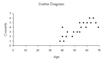A linear model appears to be appropriate to describe the relationship between the age and number of concerts attended by the respondents.
b. = -3.0115 + 0.1257x.
c. 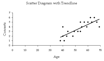d. For every additional year of age, the number of concerts attended increases by 0.1257 on average. Equivalently, we may say that for every additional 20 years of age, the number of concerts attended increases by about 2.50 on average.

A professor of economics wants to study the relationship between income y (in $1000s) and education x (in years). A random sample of eight individuals is taken and the results are shown below. Education 16 11 15 8 12 10 13 14 Income 58 40 55 35 43 41 52 49 Interpret the value of the slope of the regression line.

Free

(Essay)

4.7/5

(30)

Question 2

Correct Answer:

Verified

For each additional year of education, the income increases on average by $2909.80.

A statistician investigating the relationship between the amount of precipitation (in inches) and the number of car accidents gathered data for 10 randomly selected days. The results are presented below. Day Precipitation Number of accidents 1 0.05 5 2 0.12 6 3 0.05 2 4 0.08 4 5 0.10 8 6 0.35 14 7 0.15 7 8 0.30 13 9 0.10 7 10 0.20 10 Predict with 95% confidence the number of accidents that occur when there is 0.40 inches of rain.

Free

(Short Answer)

4.7/5

(32)

Question 3

Correct Answer:

Verified

16.316 ± 4.032 = (12.284, 20.348).

When the actual values y of a dependent variable and the corresponding predicted values $When the actual values y of a dependent variable and the corresponding predicted values are the same, the standard error of estimate, S _ { \varepsilon } , will be 0.0.$ are the same, the standard error of estimate, $S _ { \varepsilon }$ , will be 0.0.

(True/False)

4.8/5

(38)

Question 4

Test the hypothesis that the slope is significantly greater than 0.40 at the 5% level of significance.

(Essay)

4.8/5

(28)

Question 5

A regression analysis between sales (in $1000) and advertising (in $100) yielded the least squares line $A regression analysis between sales (in $1000) and advertising (in $100) yielded the least squares line = 75 +6x. This implies that if $800 is spent on advertising, then the predicted amount of sales (in dollars) is: \begin{array}{|l|l|} \hline A&\text { \$ 4,875}\\ \hline B&\text {\$ 123,000 }\\ \hline C&\text { \$ 487,500}\\ \hline D&\text { \$ 12,300}\\ \hline \end{array}$ = 75 +6x. This implies that if $800 is spent on advertising, then the predicted amount of sales (in dollars) is: A \ 4,875 B \ 123,000 C \ 487,500 D \ 12,300

(Short Answer)

4.8/5

(36)

Question 6

Which of the following statistics and procedures can be used to determine whether a linear model should be employed? A The standard error of estimate B The coefficient of determination. C The t -test of the slope. D All of these choices are correct.

(Short Answer)

4.9/5

(32)

Question 7

A financier whose specialty is investing in movie productions has observed that, in general, movies with 'big-name' stars seem to generate more revenue than those movies whose stars are less well known. To examine his belief, he records the gross revenue and the payment (in $ million) given to the two highest-paid performers in the movie for 10 recently released movies. Movie Cost of two highest- paid performers (\ ) Gross revenue (\ ) 1 5.3 48 2 7.2 65 3 1.3 18 4 1.8 20 5 3.5 31 6 2.6 26 7 8.0 73 8 2.4 23 9 4.5 39 10 6.7 58 Conduct a test of the population coefficient of correlation to determine at the 5% significance level whether a linear relationship exists between payment to the two highest-paid performers and gross revenue.

(Essay)

4.8/5

(33)

Question 8

The regression line Estimated y = 3 + 2x has been fitted to the data points (4,8), (2,5), and (1,2). The sum of the squared residuals will be: A. 7. B. 15 C. 8. D. 22.

(Short Answer)

4.8/5

(42)

Question 9

An ardent fan of television game shows has observed that, in general, the more educated the contestant, the less money he or she wins. To test her belief, she gathers data about the last eight winners of her favourite game show. She records their winnings in dollars and their years of education. The results are as follows. Contestant Years of education Winnings 1 11 750 2 15 400 3 12 600 4 16 350 5 11 800 6 16 300 7 13 650 8 14 400 Predict with 95% confidence the winnings of all contestants who have 10 years of education.

(Essay)

5.0/5

(36)

Question 10

The editor of a major academic book publisher claims that a large part of the cost of books is the cost of paper. This implies that larger books will cost more money. As an experiment to analyse the claim, a university student visits the bookstore and records the number of pages and the selling price of 12 randomly selected books. These data are listed below. Book Number of pages Selling price (\ ) 1 844 55 2 727 50 3 360 35 4 915 60 5 295 30 6 706 50 7 410 40 8 905 53 9 1058 65 10 865 54 11 677 42 12 912 58 Interpret the value of the slope of the regression line.

(Essay)

4.9/5

(39)

Question 11

A medical statistician wanted to examine the relationship between the amount of sunshine (x) and incidence of skin cancer (y). As an experiment he found the number of skin cancers detected per 100 000 of population and the average daily sunshine in eight country towns around NSW. These data are shown below. Average daily sunshine (hours) 5 7 6 7 8 6 4 3 Skin cancer per 100000 7 11 9 12 15 10 7 5 Can we conclude at the 1% significance level that there is a linear relationship between sunshine and skin cancer?

(Essay)

4.8/5

(38)

Question 12

If the standard error of estimate $S _ { \varepsilon }$ = 20 and n = 8, then the sum of squares for error, SSE, is 2400.

(True/False)

4.8/5

(41)

Question 13

The quality of oil is measured in API gravity degrees - the higher the degrees API, the higher the quality. The table shown below is produced by an expert in the field, who believes that there is a relationship between quality and price per barrel. Oil degrees API Price per barrel (in \ ) 27.0 12.02 28.5 12.04 30.8 12.32 31.3 12.27 31.9 12.49 34.5 12.70 34.0 12.80 34.7 13.00 37.0 13.00 41.0 13.17 41.0 13.19 38.8 13.22 39.3 13.27 A partial Minitab output follows. Descriptive Statistics Variable Mean StDev SE Mean Degrees 13 34.60 4.613 1.280 Frice 13 12.730 0.457 0.127 Covariances Degrees Price Degrees 21.281667 Price 2.026750 0.208833 Regression Analysis Fredictor Coef StDev Constant 9.4349 0.2867 32.91 0.000 Degrees 0.095235 0.008220 11.59 0.000 S = 0.1314 R-Sq = 92.46% R-Sq(adj) = 91.7% Analysis of Variance Source DF SS MS F P Regression 1 2.3162 2.3162 134.24 0.000 Residual Error 11 0.1898 0.0173 Total 12 2.5060 Conduct a test of the population coefficient of correlation to determine at the 5% significance level whether a linear relationship exists between the quality of oil and price per barrel.

(Essay)

4.8/5

(35)

Question 14

An ardent fan of television game shows has observed that, in general, the more educated the contestant, the less money he or she wins. To test her belief, she gathers data about the last eight winners of her favourite game show. She records their winnings in dollars and their years of education. The results are as follows. Contestant Years of education Winnings 1 11 750 2 15 400 3 12 600 4 16 350 5 11 800 6 16 300 7 13 650 8 14 400 Predict with 95% the winnings of all contestants who have 15 years of education.

(Essay)

4.7/5

(36)

Question 15

Which of the following is not a required condition for the error variable $\varepsilon$ in the simple linear regression model? A. The probability distribution of \varepsilon is normal. B. The mean of the probability distribution of \varepsilon is zero. C. The standard deviation of \varepsilon is a constant, no matter what the value of x . D. The values of \varepsilon are auto correlated.

(Short Answer)

4.9/5

(34)

Question 16

Given a specific value of x and confidence level, which of the following statements is correct? A The confidence interval estimate of the expected value of y can be calculated but the prediction interval of y for the given value of x cannot be calculated. B The confidence interval estimate of the expected value of y will be wider than the prediction interval. C The prediction interval of y for the given value of x can be calculated but the confidence interval estimate of the expected value of y cannot be calculated. D The confidence interval estimate of the expected value of y will be narrower than the prediction interval.

(Short Answer)

5.0/5

(37)

Question 17

The following sums of squares are produced: $\Sigma$ (y_i-(y-bar))² = 250, $\Sigma$ (y_i-(y_i-hat))² = 100, $\Sigma$ ((y_i-hat)-(y-bar))² = 150 The percentage of the variation in y that is explained by the variation in x is: A. 60\% B. 75\% C. 40\% D. 50\%

(Short Answer)

4.7/5

(40)

Question 18

If all the points in a scatter diagram lie on the least squares regression line, then the coefficient of correlation must be +1.0.

(True/False)

4.8/5

(27)

Question 19

Regardless of the value of x, the standard deviation of the distribution of y values about the regression line is supposed to be constant. This assumption of equal standard deviations about the regression line is called multicollinearity.

(True/False)

4.8/5

(32)

Question 20

Test the hypothesis that the slope is significantly greater than 0.40 at the 5% level of significance.

Which of the following statistics and procedures can be used to determine whether a linear model should be employed? A The standard error of estimate B The coefficient of determination. C The t -test of the slope. D All of these choices are correct.

The regression line Estimated y = 3 + 2x has been fitted to the data points (4,8), (2,5), and (1,2). The sum of the squared residuals will be: A. 7. B. 15 C. 8. D. 22.

If the standard error of estimate $S _ { \varepsilon }$ = 20 and n = 8, then the sum of squares for error, SSE, is 2400.

The following sums of squares are produced: $\Sigma$ (y_i-(y-bar))² = 250, $\Sigma$ (y_i-(y_i-hat))² = 100, $\Sigma$ ((y_i-hat)-(y-bar))² = 150 The percentage of the variation in y that is explained by the variation in x is: A. 60\% B. 75\% C. 40\% D. 50\%

If all the points in a scatter diagram lie on the least squares regression line, then the coefficient of correlation must be +1.0.

Regardless of the value of x, the standard deviation of the distribution of y values about the regression line is supposed to be constant. This assumption of equal standard deviations about the regression line is called multicollinearity.

What Is Statistics

Types of Data, Data Collection and Sampling

Graphical Descriptive Methods Nominal Data

Graphical Descriptive Techniques Numerical Data

Numerical Descriptive Measures

Probability

Random Variables and Discrete Probability Distributions

Continuous Probability Distributions

Statistical Inference: Introduction

Sampling Distributions

Estimation: Describing a Single Population

Estimation: Comparing Two Populations

Hypothesis Testing: Describing a Single Population

Hypothesis Testing: Comparing Two Populations

Inference About Population Variances

Analysis of Variance

Additional Tests for Nominal Data: Chi-Squared Tests

Multiple Regression

Model Building

Nonparametric Techniques

Statistical Inference: Conclusion

Time-Series Analysis and Forecasting

Index Numbers

Decision Analysis

Filters

Exam 18: Simple Linear Regression and Correlation

When the actual values y of a dependent variable and the corresponding predicted values are the same, the standard error of estimate, SεS _ { \varepsilon }Sε​ , will be 0.0.

Test the hypothesis that the slope is significantly greater than 0.40 at the 5% level of significance.

A regression analysis between sales (in $1000) and advertising (in $100) yielded the least squares line = 75 +6x. This implies that if $800 is spent on advertising, then the predicted amount of sales (in dollars) is: A \ 4,875 B \ 123,000 C \ 487,500 D \ 12,300

Which of the following statistics and procedures can be used to determine whether a linear model should be employed? A The standard error of estimate B The coefficient of determination. C The t -test of the slope. D All of these choices are correct.

The regression line Estimated y = 3 + 2x has been fitted to the data points (4,8), (2,5), and (1,2). The sum of the squared residuals will be: A. 7. B. 15 C. 8. D. 22.

If the standard error of estimate SεS _ { \varepsilon }Sε​ = 20 and n = 8, then the sum of squares for error, SSE, is 2400.

The following sums of squares are produced: Σ\SigmaΣ (yi-(y-bar))2 = 250, Σ\SigmaΣ (yi-(yi-hat))2 = 100, Σ\SigmaΣ ((yi-hat)-(y-bar))2 = 150 The percentage of the variation in y that is explained by the variation in x is: A. 60\% B. 75\% C. 40\% D. 50\%

If all the points in a scatter diagram lie on the least squares regression line, then the coefficient of correlation must be +1.0.

Regardless of the value of x, the standard deviation of the distribution of y values about the regression line is supposed to be constant. This assumption of equal standard deviations about the regression line is called multicollinearity.

What Is Statistics

Types of Data, Data Collection and Sampling

Graphical Descriptive Methods Nominal Data

Graphical Descriptive Techniques Numerical Data

Numerical Descriptive Measures

Probability

Random Variables and Discrete Probability Distributions

Continuous Probability Distributions

Statistical Inference: Introduction

Sampling Distributions

Estimation: Describing a Single Population

Estimation: Comparing Two Populations

Hypothesis Testing: Describing a Single Population

Hypothesis Testing: Comparing Two Populations

Inference About Population Variances

Analysis of Variance

Additional Tests for Nominal Data: Chi-Squared Tests

Multiple Regression

Model Building

Nonparametric Techniques

Statistical Inference: Conclusion

Time-Series Analysis and Forecasting

Index Numbers

Decision Analysis

Filters

If the standard error of estimate $S _ { \varepsilon }$ = 20 and n = 8, then the sum of squares for error, SSE, is 2400.

The following sums of squares are produced: $\Sigma$ (y_i-(y-bar))² = 250, $\Sigma$ (y_i-(y_i-hat))² = 100, $\Sigma$ ((y_i-hat)-(y-bar))² = 150 The percentage of the variation in y that is explained by the variation in x is: A. 60\% B. 75\% C. 40\% D. 50\%