Exam 14: Introduction to Multiple

SCENARIO 14-20-A You are the CEO of a dairy company. You are planning to expand milk production by purchasing additional cows, lands and hiring more workers. From the existing 50 farms owned by the company, you have collected data on total milk production (in liters), the number of milking cows, land size (in acres) and the number of laborers. The data are shown below and also available in the Excel file Scenario14-20-DataA.XLSX. S 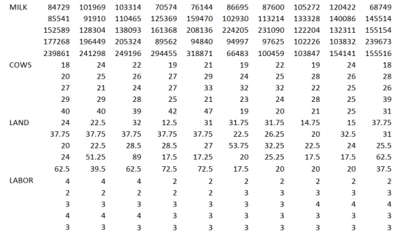You believe that the number of milking cows $\left( X _ { 1 } \right)$ , land size $\left( X _ { 2 } \right)$ and the number of laborers $\left( X _ { 3 } \right)$ are the best predictors for total milk production on any given farm. 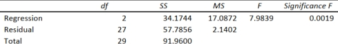-Referring to Scenario 14-20-A, what is the value of the test statistic to determine whether there is a significant relationship between total milk production and the entire set of explanatory variables?

SCENARIO 14-15 The superintendent of a school district wanted to predict the percentage of students passing a sixth- grade proficiency test. She obtained the data on percentage of students passing the proficiency test (% Passing), mean teacher salary in thousands of dollars (Salaries), and instructional spending per pupil in thousands of dollars (Spending) of 47 schools in the state. Following is the multiple regression output with $Y = \%$ Passing as the dependent variable, $X _ { 1 } =$ Salaries and $X _ { 2 } =$ Spending: Regression Statistics Multiple R 0.4276 R Square 0.1828 Adjusted R Square 0.1457 Standard Error 5.7351 Observations 47 ANOVA Coefficients Standard Error t Stat \rho -value Lower 95\% Upper 95\% Intercept -72.9916 45.9106 -1.5899 0.1190 -165.5184 19.5352 Salary 2.7939 0.8974 3.1133 0.0032 0.9853 4.6025 Spending 0.3742 0.9782 0.3825 0.7039 -1.5972 2.3455 -Referring to Scenario 14-15, the null hypothesis $H _ { 0 } : \beta _ { 1 } = \beta _ { 2 } = 0$ implies that percentage of students passing the proficiency test is not affected by either of the explanatory variables.

SCENARIO 14-18 A logistic regression model was estimated in order to predict the probability that a randomly chosen university or college would be a private university using information on mean total Scholastic Aptitude Test score (SAT) at the university or college and whether the TOEFL criterion is at least 90 (Toefl90 = 1 if yes, 0 otherwise.) The dependent variable, Y, is school type (Type = 1 if private and 0 otherwise). The PHStat output is given below: Binary Logistic Regression Predictor Coefficients SE Coef Z p -Value Intercept -3.9594 1.6741 -2.3650 0.0180 SAT 0.0028 0.0011 2.5459 0.0109 Toefl90:1 0.1928 0.5827 0.3309 0.7407 Deviance 101.9826 -Referring to Scenario 14-18, which of the following is the correct expression for the estimated model? a) $Y = - 3.9594 + 0.0028 S A T + 0.1928$ Toef 190 b) $\hat { Y } = - 3.9594 + 0.0028 S A T + 0.1928$ Toefl 90 c) $\ln ($ odds ratio $) = - 3.9594 + 0.0028 S A T + 0.1928$ Toefl 90 d) $\ln ($ estimated odds ratio $) = - 3.9594 + 0.0028$ SAT $+ 0.1928$ Toefl 90

SCENARIO 14-10 You worked as an intern at We Always Win Car Insurance Company last summer. You notice that individual car insurance premiums depend very much on the age of the individual and the number of traffic tickets received by the individual. You performed a regression analysis in EXCEL and obtained the following partial information: Regression Statistics Multiple R 0.8546 R Square 0.7303 Adjusted R Square 0.6853 Standard Error 226.7502 Observations 15 $\text { ANOVA }$ Coefficients Standard Error tStat P-value Lower 99\% Upper 99\% Intercept 821.2617 161.9391 5.0714 0.0003 326.6124 1315.9111 Age -1.4061 2.5988 -0.5411 0.5984 -9.3444 6.5321 Tickets 243.4401 43.2470 5.6291 0.0001 111.3406 375.5396 -Referring to Scenario 14-10, the estimated mean change in insurance premiums for every 2 additional tickets received is _____.

SCENARIO 14-13 An econometrician is interested in evaluating the relationship of demand for building materials to mortgage rates in Los Angeles and San Francisco. He believes that the appropriate model is $Y = 10 + 5 X _ { 1 } + 8 X _ { 2 }$ where where = mortgage rate in \% =1 if SF, 0 if LA Y= demand in \ 100 per capita -Referring to Scenario 14-13, the predicted demand in Los Angeles when the mortgage rate is 8% is ________.

SCENARIO 14-5 A microeconomist wants to determine how corporate sales are influenced by capital and wage spending by companies. She proceeds to randomly select 26 large corporations and record information in millions of dollars. The Microsoft Excel output below shows results of this multiple regression. 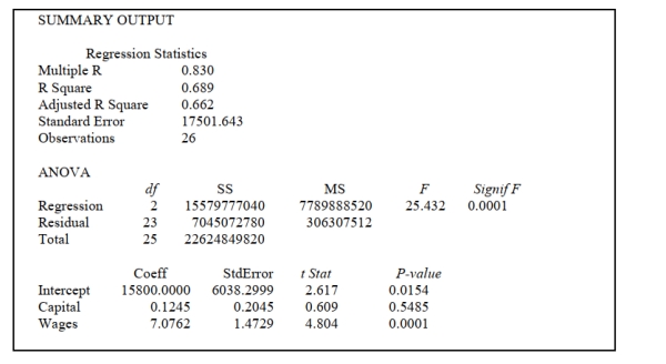-Referring to Scenario 14-5, what is the p-value for testing whether Capital has a negative influence on corporate sales?

SCENARIO 14-15 The superintendent of a school district wanted to predict the percentage of students passing a sixth- grade proficiency test. She obtained the data on percentage of students passing the proficiency test (% Passing), mean teacher salary in thousands of dollars (Salaries), and instructional spending per pupil in thousands of dollars (Spending) of 47 schools in the state. Following is the multiple regression output with $Y = \%$ Passing as the dependent variable, $X _ { 1 } =$ Salaries and $X _ { 2 } =$ Spending: Regression Statistics Multiple R 0.4276 R Square 0.1828 Adjusted R Square 0.1457 Standard Error 5.7351 Observations 47 ANOVA Coefficients Standard Error t Stat \rho -value Lower 95\% Upper 95\% Intercept -72.9916 45.9106 -1.5899 0.1190 -165.5184 19.5352 Salary 2.7939 0.8974 3.1133 0.0032 0.9853 4.6025 Spending 0.3742 0.9782 0.3825 0.7039 -1.5972 2.3455 -Referring to Scenario 14-15, what are the lower and upper limits of the 95% confidence interval estimate for the effect of a one thousand dollars increase in instructional spending per pupil on the mean percentage of students passing the proficiency test?

SCENARIO 14-20-B You are the CEO of a dairy company. You are planning to expand milk production by purchasing additional cows, lands and hiring more workers. From the existing 50 farms owned by the company, you have collected data on total milk production (in liters), the number of milking cows, land size (in acres) and the number of laborers. The data are shown below and also available in the Excel file Scenario14-20-DataB.XLSX. MILK 84686 101876 103248 70508 76072 86615 87508 105195 120351 68658 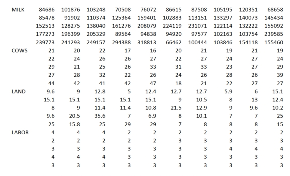You believe that the number of milking cows $\left( X _ { 1 } \right)$ , land size $\left( X _ { 2 } \right)$ and the number of laborers $\left( X _ { 3 } \right)$ are the best predictors for total milk production on any given farm. -Referring to Scenario 14-20-B, which of the following is the correct null hypothesis to test whether the number of laborers has any effect on the total milk production while holding constant The effect of the other independent variables? a) $H _ { 0 } : \beta _ { 1 } = 0$ b) $H _ { 0 } : \beta _ { 2 } = 0$ c) $H _ { 0 } : \beta _ { 3 } = 0$ d) $H _ { 0 } : \beta _ { 1 } = \beta _ { 2 } = \beta _ { 3 } = 0$

SCENARIO 14-15 The superintendent of a school district wanted to predict the percentage of students passing a sixth- grade proficiency test. She obtained the data on percentage of students passing the proficiency test (% Passing), mean teacher salary in thousands of dollars (Salaries), and instructional spending per pupil in thousands of dollars (Spending) of 47 schools in the state. Following is the multiple regression output with $Y = \%$ Passing as the dependent variable, $X _ { 1 } =$ Salaries and $X _ { 2 } =$ Spending: Regression Statistics Multiple R 0.4276 R Square 0.1828 Adjusted R Square 0.1457 Standard Error 5.7351 Observations 47 ANOVA Coefficients Standard Error t Stat \rho -value Lower 95\% Upper 95\% Intercept -72.9916 45.9106 -1.5899 0.1190 -165.5184 19.5352 Salary 2.7939 0.8974 3.1133 0.0032 0.9853 4.6025 Spending 0.3742 0.9782 0.3825 0.7039 -1.5972 2.3455 -Referring to Scenario 14-15, you can conclude definitively that instructional spending per pupil individually has no impact on the mean percentage of students passing the proficiency test, taking into account the effect of mean teacher salary, at a 1% level of significance based solely on but not actually computing the 99% the confidence interval estimate for $\beta _ { 2 }$ .

Multiple regression is the process of using several independent variables to predict a number of dependent variables.

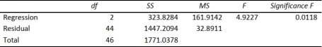
SCENARIO 14-16 What are the factors that determine the acceleration time (in sec.) from 0 to 60 miles per hour of a car? Data on the following variables for 30 different vehicle models were collected: $Y$ (Accel Time): Acceleration time in sec. $X _ { I }$ (Engine Size): c.c. $X _ { 2 }$ (Sedan): 1 if the vehicle model is a sedan and 0 otherwise The regression results using acceleration time as the dependent variable and the remaining variables as the independent variables are presented below. Regression Statistics Multiple R 0.6096 R Square 0.3716 Adjusted R Square 0.3251 Standard Error 1.4629 Observations 30 ANOVA Coefficients Standard Error t Stat P-value Lower 95\% Upper 95\% Intercept 7.1052 0.6574 10.8086 0.0000 5.7564 8.4540 Engine Size -0.0005 0.0001 -3.6477 0.0011 -0.0008 -0.0002 Sedan 0.7264 0.5564 1.3056 0.2027 -0.4152 1.8681 -Referring to Scenario 14-16, the 0 to 60 miles per hour acceleration time of a sedan is predicted to be 0.0005 seconds higher than that of a non-sedan with the same engine size.

SCENARIO 14-20-A You are the CEO of a dairy company. You are planning to expand milk production by purchasing additional cows, lands and hiring more workers. From the existing 50 farms owned by the company, you have collected data on total milk production (in liters), the number of milking cows, land size (in acres) and the number of laborers. The data are shown below and also available in the Excel file Scenario14-20-DataA.XLSX. S You believe that the number of milking cows $\left( X _ { 1 } \right)$ , land size $\left( X _ { 2 } \right)$ and the number of laborers $\left( X _ { 3 } \right)$ are the best predictors for total milk production on any given farm. 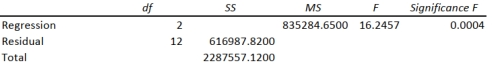-Referring to Scenario 14-20-A, what are the numerator and denominator degrees of freedom, respectively, for the test statistic to determine whether there is a significant relationship between total milk production and the entire set of explanatory variables?

SCENARIO 14-9 You decide to predict gasoline prices in different cities and towns in the United States for your term project. Your dependent variable is price of gasoline per gallon and your explanatory variables are per capita income and the number of firms that manufacture automobile parts in and around the city. You collected data of 32 cities and obtained a regression sum of squares SSR= 122.8821. Your computed value of standard error of the estimate is 1.9549. -Referring to Scenario 14-9, what is the value of the coefficient of multiple determination?

SCENARIO 14-18 A logistic regression model was estimated in order to predict the probability that a randomly chosen university or college would be a private university using information on mean total Scholastic Aptitude Test score (SAT) at the university or college and whether the TOEFL criterion is at least 90 (Toefl90 = 1 if yes, 0 otherwise.) The dependent variable, Y, is school type (Type = 1 if private and 0 otherwise). The PHStat output is given below: Binary Logistic Regression Predictor Coefficients SE Coef Z p -Value Intercept -3.9594 1.6741 -2.3650 0.0180 SAT 0.0028 0.0011 2.5459 0.0109 Toefl90:1 0.1928 0.5827 0.3309 0.7407 Deviance 101.9826 -Referring to Scenario 14-18, what should be the decision ('reject' or 'do not reject') on the null hypothesis when testing whether Toefl90 makes a significant contribution to the model in the presence of SAT at a 0.05 level of significance?