Exam 12: Multiple Regression and Model Building
Exam 1: Statistics, Data, and Statistical Thinking73 Questions
Exam 2: Methods for Describing Sets of Data194 Questions
Exam 3: Probability283 Questions
Exam 4: Discrete Random Variables133 Questions
Exam 5: Continuous Random Variables139 Questions
Exam 6: Sampling Distributions47 Questions
Exam 7: Inferences Based on a Single Sample: Estimation With Confidence Intervals124 Questions
Exam 8: Inferences Based on a Single Sample: Tests of Hypothesis140 Questions
Exam 9: Inferences Based on a Two Samples: Confidence Intervals and Tests of Hypotheses94 Questions
Exam 10: Analysis of Variance: Comparing More Than Two Means90 Questions
Exam 11: Simple Linear Regression111 Questions
Exam 12: Multiple Regression and Model Building131 Questions
Exam 13: Categorical Data Analysis60 Questions
Exam 14: Nonparametric Statistics90 Questions
Select questions type
A collector of grandfather clocks believes that the price received for the clocks at an auction increases with the number of bidders, but at an increasing (rather than a constant) rate. Thus, the model proposed to best explain auction price (y, in dollars) by number of bidders (x) is the quadratic model
This model was fit to data collected for a sample of 32 clocks sold at auction.
Suppose the -value for the test of vs. is .02. What is the proper conclusion?
A) There is evidence (at ) of upward curvature in the relationship between auction price and number of bidders .
B) There is no evidence (at ) of upward curvature in the relationship between auction price (y) and number of bidders .
C) Reject at ; the model is not useful for predicting auction price .
D) There is evidence (at ) of downward curvature in the relationship between auction price and number of bidders .
(Short Answer)
4.8/5  (25)
(25)
Consider the model where is a quantitative variable and and are dummy variables describing a qualitative variable at three levels using the coding scheme
The resulting least squares prediction equation is . What is the response line (equation) for when and ?
A)
B)
C)
D)
(Short Answer)
4.9/5 (36)
Operations managers often use work sampling to estimate how much time workers spend on each operation. Work sampling-which involves observing workers at random points in time-was applied to the staff of the catalog sales department of a clothing manufacturer. The department applied regression to the following data collected for 40 consecutive working days: TIME: Time spent (in hours) taking telephone orders during the day
ORDERS: Number of telephone orders received during the day
WEEK: weekday, 0 if Saturday or Sunday
Consider the complete 2 nd-order model:
Explain how to conduct a test to determine if a quadratic relationship between total order time and the number of orders taken is necessary in the regression model above. Specify the null and alternative hypotheses that are to be tested.
(Essay)
4.9/5 (36)
In the presence of multicollinearity, you should avoid making inferences about the parameters based on the t-tests.
(True/False)
5.0/5 (42)
The printout below shows part of the least squares regression analysis for the model fit to a set of data. The model attempts to predict a score on the final exam in a statistics course based on the scores on the first two tests in the class. ANOVA df SS MS F Significance F Regression 2 1293.125328 646.5626641 21.27366772 2.35769-05 Residual 17 516.6746719 30.39262776 Total 19 1809.8 Coefficients Standard Error t Stat P-value Lower 95\% Upper 95\% Intercept -4.409686163 16.72267106 -0.263695085 0.795184685 -39.69148734 30.87211502 Test 1 0.397435806 0.343012569 1.158662514 0.262611745 -0.326258467 1.121130079 Test 2 0.638805278 0.224623383 2.843894834 0.011217936 0.164890704 1.112719852 Is there evidence of multicollinearity in the printout? Explain.
(Essay)
4.8/5 (38)
As part of a study at a large university, data were collected on n = 224 freshmen computer science (CS) majors in a particular year. The researchers were interested in modeling y, a student's grade point average (GPA) after three semesters, as a function of the following independent variables (recorded at the time the students enrolled in the university): = average high school grade in mathematics (HSM) = average high school grade in science (HSS) = average high school grade in English (HSE) = SAT mathematics score (SATM) = SAT verbal score (SATV)
SOURCE DF SS MS F VALUE PROB > F MODEL 5 28.64 5.73 11.69 .0001 ERROR 218 106.82 0.49 TOTAL 223 135.46
ROOT MSE 0.700 R-SQUARE 0.211 DEP MEAN 4.635 ADJ R-SQ 0.193
PARAMETER STANDARD TFOR O: VARIABLE ESTIMATE ERROR PARAMETER =0 PROB >|T| INTERCEPT 2.327 0.039 5.817 0.0001 X1 (HSM) 0.146 0.037 3.718 0.0003 X2 (HSS) 0.036 0.038 0.950 0.3432 X3 (HSE) 0.055 0.040 1.397 0.1637 X4 (SATM) 0.00094 0.00068 1.376 0.1702 X5 (SATV) -0.00041 0.0059 -0.689 0.4915
(Essay)
4.8/5 (35)
Consider the second-order model
If is held fixed at , describe the relationship between and .
A) The relationship between and is quadratic with upward concavity.
B) The relationship between and is quadratic with downward concavity.
C) The relationship between and is linear with positive slope.
D) The relationship between and is linear with negative slope.
(Short Answer)
4.8/5 (41)
The complete second-order model with two quantitative independent variables does not allow for interaction between the two independent variables.
(True/False)
4.9/5 (27)
The concessions manager at a beachside park recorded the high temperature, the number of people at the park, and the number of bottles of water sold for each of 12 consecutive Saturdays. The data are shown below. Bottles Sold Temperature People 341 73 1625 425 79 2100 457 80 2125 485 80 2800 469 81 2550 395 82 1975 511 83 2675 549 83 2800 543 85 2850 537 88 2775 621 89 2800 897 91 3100 a. Fit the model to the data, letting y represent the number of bottles of water sold, x1 the temperature, and x2 the number of people at the park. b. Identify at least two indicators of multicollinearity in the model. c. Comment on the usefulness of the model to predict the number of bottles of water sold on a Saturday when the high temperature is 103°F and there are 3500 people at the park.
(Essay)
4.9/5 (31)
As part of a study at a large university, data were collected on n = 224 freshmen computer science (CS) majors in a particular year. The researchers were interested in modeling y, a student's grade point average (GPA) after three semesters, as a function of the following independent variables (recorded at the time the students enrolled in the university): average high school grade in mathematics (HSM)
average high school grade in science (HSS)
average high school grade in English (HSE)
SAT mathematics score (SATM)
SAT verbal score (SATV)
A first-order model was fit to data with .
What is the correct interpretation of , the coefficient of determination for the model?
A) Approximately of the sample variation in GPAs can be explained by the first-order model.
B) We expect to predict GPA to within approximately .21 of its true value.
C) Approximately of the sample variation in GPAs can be explained by the first-order model.
D) We are confident that the model is useful for predicting .
(Short Answer)
4.8/5 (38)
In regression, it is desired to predict the dependent variable based on values of other related independent variables. Occasionally, there are relationships that exist between the independent variables. Which of the following multiple regression pitfalls does this example describe?
(Multiple Choice)
4.8/5 (39)
A study of the top MBA programs attempted to predict y = the average starting salary (in $1000's) of graduates of the program based on x = the amount of tuition (in $1000's) charged by the program. After first considering a simple linear model, it was decided that a quadratic model should be proposed. Which of the following models proposes a 2nd-order quadratic relationship between x and y? A)
B)
C)
D)
(Short Answer)
4.9/5 (36)
Why is the random error term ε added to a multiple regression model? 12.2 Estimating and Making Inferences about the β Parameters 1 Write First-Order Model
(Essay)
4.8/5 (31)
In the first-order model represents the slope of the line relating to when and are both held fixed.
(True/False)
4.8/5 (40)
Stepwise regression is used to determine which variables, from a large group of variables, are useful in predicting the value of a dependent variable.
(True/False)
4.7/5 (40)
The complete second-order model data points. The printout is shown below.
df SS MS F Significance F Regression 5 22812.46538 4562.493077 56487.98 6.12671-39 Residual 19 1.534616187 0.080769273 Total 24 22814
Coefficients Standard Error t Stat P-value Lower 95\% Upper 95\% Intercept -0.202274307 0.377603882 -0.535678569 0.598396064 -0.99260856 0.588059946 1 0.57956491 0.184697537 3.137913578 0.005416889 0.192988402 0.966141418 2 0.502983937 0.130940123 3.841327815 0.001100855 0.228923024 0.777044849 2 1.976110807 0.022011043 89.77815357 1.92982-26 1.93004115 2.022180464 2 -0.026825292 0.025350994 -1.058155454 0.303252905 -0.079885548 0.026234964 2 0.012944358 0.015088978 0.857868446 0.401657492 -0.018637245 0.044525961 a. Write the complete second-order model for the data.
b. Is there sufficient evidence to indicate that at least one of the parameters , and is nonzero?
Test using .
c. Test against . Use .
d. Test against . Use . 3 Test if Model is Useful for Predicting y
(Essay)
4.8/5 (32)
What relationship between x and y is suggested by the scattergram? 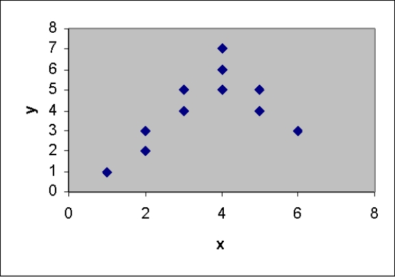
(Multiple Choice)
4.7/5 (28)
The stepwise regression procedure may not be used when the inclusion of one or more dummy variables is under consideration.
(True/False)
4.7/5 (36)
In Hawaii, proceedings are under way to enable private citizens to own the property that their homes are built on. In prior years, only estates were permitted to own land, and homeowners leased the land from the estate. In order to comply with the new law, a large Hawaiian estate wants to use regression analysis to estimate the fair market value of the land. The following variables are proposed: Sale price of property ( thousands)
if property near Cove, 0 if not Write a regression model relating the sale price of a property to the qualitative variable x. Interpret all the βs in the model.
(Essay)
4.9/5 (39)
Filters
- Essay(0)
- Multiple Choice(0)
- Short Answer(0)
- True False(0)
- Matching(0)