Exam 12: Multiple Regression and Model Building

A certain type of rare gem serves as a status symbol for many of its owners. In theory, for low prices, the demand decreases as the price of the gem increases. However, experts hypothesize that when the gem is valued at very high prices, the demand increases with price due to the status the owners believe they gain by obtaining the gem. Thus, the model proposed to best explain the demand for the gem by its price is the quadratic model $E ( y ) = \beta _ { 0 } + \beta _ { 1 } x + \beta _ { 2 } x ^ { 2 }$ where $y =$ Demand (in thousands) and $x =$ Retail price per carat (dollars). This model was fit to data collected for a sample of 12 rare gems. A portion of the printout is given below: SOURCE DF SS MS F PR > F Model 2 115145 57573 373 .0001 Error 9 1388 154 TOTAL 11 116533 Root MSE $\quad 12.42 \quad$ R-Square $\quad .988$ PARAMETER T for $\mathrm { HO }$ : \begin{array} { l r r r r }& \text {PARAMETER}&& \text { \mathrm{T} for \( \mathrm{HO} \) }:\\\text {VARIABLES}& \text {ESTIMATES }& \text {STD. ERROR}& \text { PARAMETER = 0 }& \text {PR \(> | T |\)}\\ \text { INTERPCEP } & 286.42 & 9.66 & 29.64 & .0001 \\ \mathrm { X } & - .31 & .06 & - 5.14 & .0006 \\ \mathrm { X } \cdot \mathrm { X } & .000067 & .00007 & .95 & .3647 \end{array} Is there sufficient evidence to indicate the model is tuseful for predicting the demand for the gem? Use $\alpha = .01$ .

The value of R2 is only useful when the number of data points is substantially larger than the number of β parameters in the model.

Residual analysis can be used to check for violations of the assumptions that the distribution of the random error component is normally distributed with mean 0.

As part of a study at a large university, data were collected on n = 224 freshmen computer science (CS) majors in a particular year. The researchers were interested in modeling y, a student's grade point average (GPA) after three semesters, as a function of the following independent variables (recorded at the time the students enrolled in the university): $x _ { 1 } =$ average high school grade in mathematics (HSM) $x _ { 2 } =$ average high school grade in science (HSS) $x _ { 3 } =$ average high school grade in English (HSE) $x _ { 4 } =$ SAT mathematics score (SATM) $x _ { 5 } =$ SAT verbal score (SATV) A first-order model was fit to data with the following results: SOURCE DF SS MS FVALUE PROB > F MODEL 5 28.64 5.73 11.69 .0001 ERROR 218 106.82 0.49 TOTAL 223 135.46 ROOT MSE 0.700 R-SOUARE 0.211 DEP MEAN 4.635 ADJ R-5Q 0.193 PARAMETER STANDARD T FOR O: VARIABLE ESTIMATE ERROR PARAMETER =0 PROB >|T| INTERCEPT 2.327 0.039 5.817 0.0001 X1 (HSM) 0.146 0.037 3.718 0.0003 X2 (HSS) 0.036 0.038 0.950 0.3432 X3 (HSE) 0.055 0.040 1.397 0.1637 X4 (SATM) 0.00094 0.00068 1.376 0.1702 X5 (SATV) -0.00041 0.00059 -0.689 0.4915 Interpret the value under the column heading $\mathrm { PROB } > \mathrm { F }$ . A) There is sufficient evidence (at $\alpha = .01$ ) to conclude that the first-order model is statistically useful for predicting GPA. B) There is insufficient evidence (at $\alpha = .01$ ) to conclude that the first-order model is statistically useful for predicting GPA. C) Over $99 \%$ of the variation in GPAs can be explained by the model. D) Accept $H _ { 0 }$ (at $\alpha = .01$ ); at least one of the $\beta$ -coefficients in the first-order model is equal to 0 .

The concessions manager at a beachside park recorded the high temperature, the number of people at the park, and the number of bottles of water sold for each of 12 consecutive Saturdays. The data are shown below. Bottles Sold Temperature People 341 73 1625 425 79 2100 457 80 2125 485 80 2800 469 81 2550 395 82 1975 511 83 2675 549 83 2800 543 85 2850 537 88 2775 621 89 2800 897 91 3100 a. Fit the model $E ( y ) = \beta _ { 0 } + \beta _ { 1 } x _ { 1 } + \beta _ { 2 } x _ { 2 }$ to the data, letting $y$ represent the number of bottles of water sold, $x _ { 1 }$ the temperature, and $x _ { 2 }$ the number of people at the park. b. Find the $95 \%$ confidence interval for the mean number of bottles of water sold when the temperature is $84 ^ { \circ } \mathrm { F }$ and there are 2700 people at the park. c. Find the $95 \%$ prediction interval for the number of bottles of water sold when the temperature is $84 ^ { \circ } \mathrm { F }$ and there are 2700 people at the park. 12.5 Interaction Models 1 Write Interaction Model

A regression residual is the difference between an observed y value and its corresponding predicted value.

During its manufacture, a product is subjected to four different tests in sequential order. An efficiency expert claims that the fourth (and last) test is unnecessary since its results can be predicted based on the first three tests. To test this claim, multiple regression will be used to model Test 4 score (y), as a function of Test1 score $\left( x _ { 1 } \right)$ , Test 2 score $\left( x _ { 2 } \right)$ , and Test3 score $\left( x _ { 3 } \right)$ . [Note: All test scores range from 200 to 800 , with higher scores indicative of a higher quality product.] Consider the model: $E ( y ) = \beta _ { 1 } + \beta _ { 1 } x _ { 1 } + \beta _ { 2 } x _ { 2 } + \beta _ { 3 } x _ { 3 }$ The global $F$ statistic is used to test the null hypothesis, $H _ { 0 } : \beta _ { 1 } = \beta _ { 2 } = \beta _ { 3 } = 0$ . Describe this hypothesis in words.

The model $E ( y ) = \beta _ { 0 } + \beta _ { 1 } x$ x was fit to a set of data, and the following plot of residuals against x values was obtained. 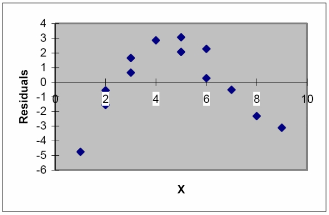Interpret the residual plot.

A college admissions officer proposes to use regression to model a student's college GPA at graduation in terms of the following two variables: = high school GPA = SAT score The admissions officer believes the relationship between college GPA and high school GPA is linear and the relationship between SAT score and college GPA is linear. She also believes that the relationship between college GPA and high school GPA depends on the student's SAT score. Write the regression model she should fit. 2 Test if Model is Useful for Predicting y

Retail price data for n = 60 hard disk drives were recently reported in a computer magazine. Three variables were recorded for each hard disk drive: $y =$ Retail PRICE (measured in dollars) $x _ { 1 } =$ Microprocessor SPEED (measured in megahertz) (Values in sample range from 10 to 40 ) $x _ { 2 } = \mathrm { CHIP }$ size (measured in computer processing units) (Values in sample range from 286 to 486 ) A first-order regression model was fit to the data. Part of the printout follows: Parameter Estimates PARAMETER STANDARD T FOR 0: VARIABLE DF ESTIMATE ERROR PARAMETER =0 PROB > |T| = INTERCEPT 1 -373.526392 1258.1243396-0.297 0.7676 SPEED 1 104.838940 22.362981954.688 0.0001 CHIP 1 3.571850 3.894229350.917 0.3629 Identify and interpret the estimate for the SPEED $\beta$ -coefficient, $\hat { \beta } _ { 1 }$ . A) $\hat { \beta } _ { 1 } = 105$ ; For every 1-megahertz increase in SPEED, we estimate PRICE $( y )$ to increase $\$ 105$ , holding CHIP fixed. B) $\hat { \beta } _ { 1 } = 105$ ; For every $\$ 1$ increase in PRICE, we estimate SPEED to increase 105 megahertz, holding CHIP fixed. C) $\hat { \beta } _ { 1 } = 3.57 ;$ For every 1 -megahertz increase in SPEED, we estimate PRICE to increase $\$ 3,57$ , holding CHIP fixed. D) $\hat { \beta } _ { 1 } = 3.57$ ; For every $\$ 1$ increase in PRICE, we estimate SPPED to increase by about 4 megahertz, holding CHIP fixed.

A collector of grandfather clocks believes that the price received for the clocks at an auction increases with the number of bidders, but at an increasing (rather than a constant) rate. Thus, the model proposed to best explain auction price (y, in dollars) by number of bidders (x) is the quadratic model $E ( y ) = \beta _ { 0 } + \beta _ { 1 } x + \beta _ { 2 } x ^ { 2 }$ This model was fit to data collected for a sample of 32 clocks sold at atiction; a portion of the printout follows: SOURCE DF 55 MS FVALUE PROB > F MODEL 2 4277160 2138579 120 .0005 ERROR 29 514034 17725 TOTAL 31 4791194 ROOT MSE 133 R-SQUARE 893 DEP MEAN 1327 ADJ R-SQ .885 PARAMETER STANDARD T FOR 0: VARIABLES ESTIMATE ERROR PARAMETER =0 PROB >|T| INTERCEPT 286.42 9.66 29.64 .0001 .31 .06 5.14 .0016 \cdot -.000067 .00007 -0.95 .3600 An outlier for the model is a clock with a residual that _____ in absolute value. (Fill in the blank.)

A certain type of rare gem serves as a status symbol for many of its owners. In theory, for low prices, the demand decreases as the price of the gem increases. However, experts hypothesize that when the gem is valued at very high prices, the demand increases with price due to the status the owners believe they gain by obtaining the gem. Thus, the model proposed to best explain the demand for the gem by its price is the quadratic model $E ( y ) = \beta _ { 0 } + \beta _ { 1 } x + \beta _ { 2 } x ^ { 2 }$ where $y =$ Demand (in thousands) and $x =$ Retail price per carat (dollars). This model was fit to data collected for a sample of 12 rare gems. A portion of the printout is given below: SOURCE DF 55 M5 F PR > F Model 2 115145 57573 373 ,0001 Error 9 1388 154 TOTAL 11 116533 $\text { Root MSE } \quad 12.42 \quad \text { R-Square } \quad 988$ VARIABLES ESTIMATES STD, ERROR PARAMETER =0 P R>|T| INTERPCEP 286.42 9.66 29.64 .0001 -.31 .06 -5.14 .0006 \cdot .000067 .00007 .95 .3647 Does the quadratic term contribute useful information for predicting the demand for the gem? Use $\alpha = .10$ .

It is desired to build a regression model to predict $\mathrm { y } =$ the sales price of a single family home, based on the $\mathrm { x } _ { 1 } =$ size of the house and $x _ { 2 } =$ the neighborhood the home is located in. The goal is to compare the prices of homes that are located in two different neighborhoods. A complete 2nd-order model is proposed. Which regression model proposes the complete 2nd-order model? A) $E(y)=\beta_{0}+\beta_{1} x_{1}+\beta_{2} x_{2}$ B) $E(y)=\beta_{0}+\beta_{1} x_{1}+\beta_{2} x_{2}+\beta_{3} x_{1} x_{2}$ C) $E(y)=\beta_{0}+\beta_{1} x_{1}+\beta_{2} x_{1}^{2}+\beta_{3} x_{2}+\beta_{4} x_{2}{ }^{2}$ D) $E(y)=\beta_{0}+\beta_{1} x_{1}+\beta_{2} x_{1}^{2}+\beta_{3} x_{2}+\beta_{4} x_{1} x_{2}+\beta_{3} x_{1}^{2} x_{2}$

The model $E ( y ) = \beta _ { 0 } + \beta _ { 1 } x _ { 1 } + \beta _ { 2 } x _ { 2 } + \beta _ { 3 } x _ { 3 } + \beta _ { 4 } x _ { 4 }$ was used to relate $E ( y )$ to a single qualitative variable, where = 1 if level 2 0 if not = 1 if level 3 0 if not = 1 if level 4 0 if not 1 if level 5 0 if not This model was fit to $n = 40$ data points and the following result was obtained: $\hat { y } = 14.5 + 3 x _ { 1 } - 4 x _ { 2 } + 10 x _ { 3 } + 8 x _ { 4 }$ a. Use the least squares prediction equation to find the estimate of $E ( y )$ for each level of the qualitative variable. b. Specify the null and alternative hypothesis you would use to test whether $E ( y )$ is the same for all levels of the independent variable. 3 Test if Model is Useful for Predicting y

Once interaction has been established between $x _ { 1 }$ and $x _ { 2 }$ , the first-order terms for $x _ { 1 }$ and $x _ { 2 }$ may be deleted from the regression model leaving the higher-order term containing the product of $x _ { 1 }$ and $x _ { 2 }$ .

Consider the model $y = \beta _ { 0 } + \beta _ { 1 } x _ { 1 } + \beta _ { 2 } x _ { 1 }^{ 2} + \beta _ { 3 } x _ { 2 } + \beta _ { 4 } x _ { 3 } + \beta _ { 5 } x _ { 1 } x _ { 2 } + \beta _ { 6 } x _ { 1 } x _ { 3 } + \beta _ { 7 } x _ { 1 }^{ 2} { x _ { 2 } } + \beta _ { 8 } x _ { 1 }^{ 2} { x _ { 3 } } + \varepsilon$ where $x _ { 1 }$ is a quantitative variable and $x _ { 2 }$ and $x _ { 3 }$ are dummy variables describing a qualitative variable at three levels using the coding scheme $x _ { 2 } = \left\{ \begin{array} { l l } 1 & \text { if level } 2 \\0 & \text { otherwise }\end{array} \quad x _ { 3 } = \left\{ \begin{array} { l l } 1 & \text { if level } 3 \\0 & \text { otherwise }\end{array} \right. \right.$ The resulting least squares prediction equation is $\hat { y } = 8.8 - 1.1 x _ { 1 } + 3.2 x _ { 1 } ^ { 2 } + 1.6 x _ { 2 } - 4.4 x _ { 3 } + .02 x _ { 1 } x _ { 2 } + 1.3 x _ { 1 } x _ { 3 } + .01 x _ { 1 } { } ^ { 2 } x _ { 2 } - .06 x _ { 1 }^{2} x _ { 3 }$ What is the equation of the response curve for $E ( y )$ when $x _ { 2 } = 0$ and $x _ { 3 } = 0$ ? A) $\hat { y } = 8.8 - 1.1 x _ { 1 } + 3.2 x _ { 1 } { } ^ { 2 }$ B) $\hat { y } = 8.8 - 1.3 x _ { 1 } + 3.2 x _ { 1 } { } ^ { 2 }$ C) $y = 8.8 - .22 x _ { 1 } + 3.15 x _ { 1 } { } ^ { 2 }$ D) $y = 8.8 - 1.6 x _ { 2 } - 4.4 x _ { 3 }$

The method of fitting first-order models is the same as that of fitting the simple straight-line model, i.e. the method of least squares.

The model $E ( y ) = \beta _ { 0 } + \beta _ { 1 } x _ { 1 } + \beta _ { 2 } x _ { 2 } + \beta _ { 3 } x _ { 3 }$ was used to relate E(y) to a single qualitative variable. How many levels does the qualitative variable have?

The sum of squared errors (SSE) of a least squares regression model decreases when new terms are added to the model.

The model $E ( y ) = \beta _ { 0 } + \beta _ { 1 } x$ was fit to a set of data, and the following plot of residuals against x values was obtained. 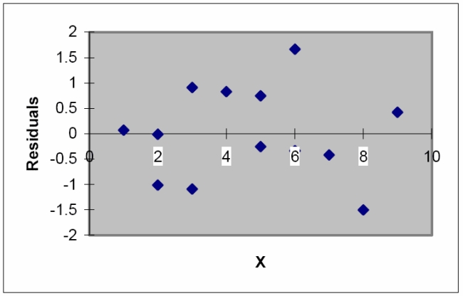Interpret the residual plot.