Exam 12: Multiple Regression and Model Building

A graphing calculator was used to fit the model E(y) = ?0 + ?1x + ?2x2 to a set of data. The resulting screen is shown below. 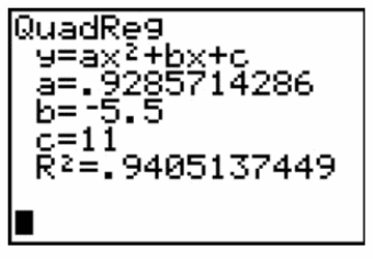Which number on the screen represents the estimator of $\beta _ { 2 }$ ?

It is desired to build a regression model to predict y = the sales price of a single family home, based on the neighborhood the home is located in. The goal is to compare the prices of homes that are located in four different neighborhoods. Which regression model should be built? A) $E ( y ) = \beta _ { 0 } + \beta _ { 1 } x _ { 1 } + \beta _ { 2 } x _ { 2 } + \beta _ { 3 } x _ { 3 } + \beta _ { 4 } x _ { 4 }$ , where $x _ { 1 } - x _ { 4 }$ are qualitative variables that describe the four neighborhoods. B) $\mathrm { E } ( \mathrm { y } ) = \beta _ { 0 } + \beta _ { 1 } \mathrm { x } _ { 1 } + \beta _ { 2 } \mathrm { x } _ { 2 } + \beta _ { 3 } \mathrm { x } _ { 3 }$ , where $\mathrm { x } _ { 1 } - \mathrm { x } _ { 3 }$ are qualitative variables that describe the four neighborhoods. C) $\mathrm { E } ( \mathrm { y } ) = \beta _ { 0 } + \beta _ { 1 } \mathrm { x } _ { 1 }$ , where $\mathrm { x } _ { 1 }$ is a qualitative variable that describes the four neighborhoods. D) $\mathrm { E } ( \mathrm { y } ) = \beta _ { 0 } + \beta _ { 1 } \mathrm { x } _ { 1 } + \beta _ { 2 } \mathrm { x } _ { 1 } { } ^ { 2 }$ , where $\mathrm { x } _ { 1 }$ is a qualitative variable that describes the four neighborhoods.

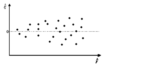
Suppose that the following model was fit to a set of data. $E ( y ) = \beta _ { 0 } + \beta _ { 1 } x _ { 1 } + \beta _ { 2 } x _ { 2 }$ The corresponding plot if residuals against predicted values $\hat{y}$ is shown. Interpret the plot.

A first-order model may include terms for both quantitative and qualitative independent variables.

A collector of grandfather clocks believes that the price received for the clocks at an auction increases with the number of bidders, but at an increasing (rather than a constant) rate. Thus, the model proposed to best explain auction price (y, in dollars) by number of bidders (x) is the quadratic model $E ( y ) = \beta _ { 0 } + \beta _ { 1 } x + \beta _ { 2 } x ^ { 2 }$ This model was fit to data collected for a sample of 32 clocks sold at atiction; the restilting estimate of $\beta _ { 1 }$ was $- 31$ . Interpret this estimate of $\beta _ { 1 }$ . A) $\beta _ { 1 }$ is a shift parameter that has no practical interpretation. B) We estimate the auction price will decrease $\$ .31$ for each additional bidder at the atiction. C) We estimate the auction price will increase $\$ .31$ for each additional bidder at the auction. D) We estimate the auction price will be $- \$ .31$ when there are no bidders at the atuction.

It is desired to build a regression model to predict $\mathrm { y } =$ the sales price of a single family home, based on the $\mathrm { x } _ { 1 } =$ size of the house and $\mathrm { x } _ { 2 } =$ the neighborhood the home is located in. The goal is to compare the prices of homes that are located in two different neighborhoods. The following model is proposed: $E ( y ) = \beta _ { 0 } + \beta _ { 1 } x _ { 1 } + \beta _ { 2 } x _ { 2 }$ A regression model was fit and the following residual plot was observed. 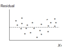Which of the following assumptions appears violated based on this plot?

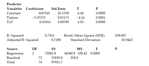
A study of the top MBA programs attempted to predict the average starting salary (in $1000's) of graduates of the program based on the amount of tuition (in $1000's) charged by the program and the average GMAT score of the program's students. The results of a regression analysis based on a sample of 75 MBA programs is shown below: Least Squares Linear Regression of Salary Predictor Cases Included 75 Missing Cases 0 The global-f test statistic is shown on the printout to be the value $\mathrm { F } = 100.42$ . Interpret this value. A) There is insufficient evidence, at $\alpha = 0.05$ , to indicate that at least one of the variables proposed in the interaction model is useful at predicting the average starting salary of graduates of MBA programs. B) There is sufficient evidence, at $\alpha = 0.05$ , to indicate that at least one of the variables proposed in the interaction model is useful at predicting the average starting salary of graduates of MBA programs. C) There is sufficient evidence, at $\alpha = 0.05$ , to indicate that there is a curvilinear relationship between average starting salary of graduates of MBA programs and the tuition of the MBA program. D) There is sufficient evidence, at $\alpha = 0.05$ , to indicate that there is a linear relationship between average starting salary of graduates of MBA programs and the tuition of the MBA program.

A certain type of rare gem serves as a status symbol for many of its owners. In theory, for low prices, the demand decreases as the price of the gem increases. However, experts hypothesize that when the gem is valued at very high prices, the demand increases with price due to the status the owners believe they gain by obtaining the gem. Thus, the model proposed to best explain the demand for the gem by its price is the quadratic model $E ( y ) = \beta _ { 0 } + \beta _ { 1 } x + \beta _ { 2 } x ^ { 2 }$ where $y =$ Demand (in thousands) and $x =$ Retail price per carat (dollars). This model was fit to data collected for a sample of 12 rare gems. VARIABLES PARAMETER ESTIMATES STD. ERROR T for HO: PARAMETER =0 PR >|T| INTERPCEP 286.42 9.66 X -.31 .06 29.64 .0001 X.X .000067 .00007 -5.14 .0006 .95 .3647 Does there appear to be upward curvature in the response curve relating $y$ (demand) to $x$ (retail price)? A) No, since the $p$ -value for the test is greater than .10. B) Yes, since the $p$ -value for the test is less than .01. C) No, since the value of $\beta _ { 2 }$ is near 0 . D) Yes, since the value of $\beta _ { 2 }$ is positive.

When using the model E(y) = β0 + β1x for one qualitative independent variable with a 0-1 coding convention, β1 represents the difference between the mean responses for the level assigned the value 1 and the base level.

The stepwise regression model should not be used as the final model for predicting y.

During its manufacture, a product is subjected to four different tests in sequential order. An efficiency expert claims that the fourth (and last) test is unnecessary since its restults can be predicted based on the first three tests. To test this claim, multiple regression will be used to model Test 4 score (y), as a function of Test1 score $\left( x _ { 1 } \right)$ . Test 2 score $\left( x _ { 2 } \right)$ , and Test 3 score $\left( x _ { 3 } \right)$ . [Note: All test scores range from 200 to 800 , with higher scores indicative of a higher quality product.] Consider the model: $E ( y ) = \beta _ { 1 } + \beta _ { 1 } x _ { 1 } + \beta _ { 2 } x _ { 2 } + \beta _ { 3 } x _ { 3 }$ The first-order model was fit to the data for each of 12 units sampled from the production line. The results are summarized in the printout. A) $.33 \pm .19$ B) $33 \pm 105$ C). $.33 \pm .08$ D) $.33 \pm 4.04$

An elections officer wants to model voter turnout (y) in a precinct as a function of type of election, national or state. Write a model for mean voter turnout, E(y), as a function of type of election. A) $E ( y ) = \beta _ { 0 } + \beta _ { 1 } x$ , where $x = 1$ if national, 0 if state B) $E ( y ) = \beta _ { 0 } + \beta _ { 1 } x _ { 1 } + \beta _ { 2 } x _ { 2 }$ , where $x _ { 1 } = 1$ if national, 0 if not and $x _ { 2 } = 1$ if state, 0 if not C) $E ( y ) = \beta _ { 0 } + \beta _ { 1 } x$ , where $x =$ voter turnout D) $E ( y ) = \beta _ { 0 } + \beta _ { 1 } x + \beta _ { 2 } x ^ { 2 }$ , where $x =$ voter turnout

A study of the top MBA programs attempted to predict the average starting salary (in $1000's) of graduates of the program based on the amount of tuition (in $1000's) charged by the program and the average GMAT score of the program's students. The results of a regression analysis based on a sample of 75 MBA programs is shown below: Least Squares Linear Regression of Salary 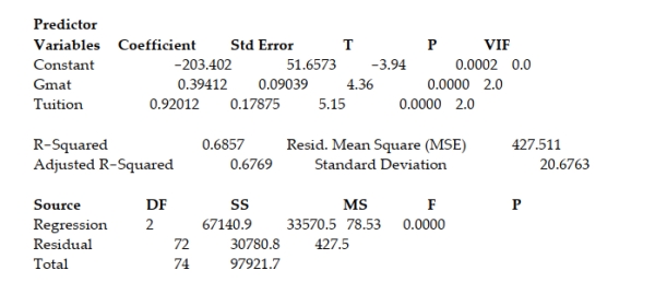Interpret the coefficient of determination value shown in the printout.

Consider the data given in the table below. 1 4 2 6 2 5 3 7 4 7 4 6 5 4 5 5 6 3 a. Plot the data on a scattergram. Does a quadratic model seem to be a good fit for the data? Explain. b. Use the method of least squares to find a quadratic prediction equation. c. Graph the prediction equation on your scattergram. 12.7 Qualitative (Dummy) Variable Models 1 Write and Interpret Model with Qualitative Variables

The staff of a test kitchen is attempting to determine the baking time, y, of a roast, i.e., the time it takes the internal temperature of the roast to reach 165°F, using two variables, the temperature setting of the oven, x1, and the weight of the roast, x2, in pounds. The data for 24 roasts are shown below. $\text { Baking Times of Roasts }$ 1 2() () 1 2() () 1 2() () 1 2() () 300 2.2 2.6 325 2.1 2.3 350 2.3 2.2 375 2.2 1.9 300 2.7 2.8 325 2.4 2.4 350 2.5 2.3 375 2.6 2.2 300 2.9 3.1 325 2.9 2.6 350 2.8 2.5 375 2.9 2.4 300 3.1 3.2 325 3.0 2.7 350 3.2 2.7 375 3.1 2.6 300 3.2 3.2 325 3.2 2.9 350 3.4 2.8 375 3.3 2.7 300 3.5 3.3 325 3.6 3.1 350 3.5 2.8 375 3.4 2.7 a. Fit a complete second-order model to the data. b. Do the data provide sufficient evidence to indicate that the second-order terms contribute information for the prediction of y? State the null and alternative hypotheses and the test statistic. Use α = .05. 12.10 Stepwise Regression (Optional) 1 Understand and Interpret Stepwise Regression Model

The number of levels of observed x-values must be equal to the order of the polynomial in x that you want to fit.

Which of the following is not a possible indicator of multicollinearity?

A nested model F-test can only be used to determine whether second-order terms should be included in the model.

Consider the partial printout for an interaction regression analysis of the relationship between a dependent variable y and two independent variables x1 and x2. ANOVA df SS MS F Significance F Regression 3 3393.677324 1131.225775 9391.974782 2.11084-11 Residual 6 0.722675987 0.120445998 Total 9 3394.4 Coefficients Standard Error t Stat P-value Lower 95\% Upper 95\% Intercept 16.72197014 8.283997219 2.018587126 0.09007654 -3.548255659 36.99219593 X1 -3.037317759 2.678748705 -1.133856921 0.300116382 -9.591984506 3.517348987 X2 -1.046522754 1.547132645 -0.676427297 0.523973988 -4.832222727 2.73917722 X1X2 4.071685147 0.444059933 9.169224345 9.47663-05 2.98510884 5.158261454 a. Write the prediction equation for the interaction model. b. Test the overall utility of the interaction model using the global $F$ -test at $\alpha = .05$ . c. Test the hypothesis (at $\alpha = .05$ ) that $x _ { 1 }$ and $x _ { 2 }$ interact positively. d. Estimate the change in $y$ for each additional 1-unit increase in $x _ { 1 }$ when $x _ { 2 } = 6$ . 3 Test for Interaction Between Two Variables

If when using the model $E ( y ) = \beta _ { 0 } + \beta _ { 1 } x _ { 1 } + \beta _ { 2 } x _ { 2 } + \beta _ { 3 } x _ { 1 } x _ { 2 }$ we determine that interaction between $x _ { 1 }$ and $x _ { 2 }$ is not significant, we can drop the $x _ { 1 } x _ { 2 }$ term from the model and use the simpler model $E ( y ) = \beta _ { 0 } + \beta _ { 1 } x _ { 1 } + \beta _ { 2 } x _ { 2 }$