Exam 12: Multiple Regression and Model Building

In stepwise regression, the probability of making one or more Type I or Type II errors is quite small.

A certain type of rare gem serves as a status symbol for many of its owners. In theory, for low prices, the demand decreases as the price of the gem increases. However, experts hypothesize that when the gem is valued at very high prices, the demand increases with price due to the status the owners believe they gain by obtaining the gem. Thus, the model proposed to best explain the demand for the gem by its price is the quadratic model $E ( y ) = \beta _ { 0 } + \beta _ { 1 } x + \beta _ { 2 } x ^ { 2 }$ where $y =$ Demand (in thousands) and $x =$ Retail price per carat (dollars). This model was fit to data collected for a sample of 12 rare gems. If the experts are correct in their assumptions about the relationship between price and demand, which of the following should be true? A) $\beta _ { 2 } > 0$ B) $\beta _ { 2 } < 0$ C) $\beta _ { 1 } > 0$ D) $\beta _ { 1 } < 0$

We expect all or almost all of the residuals to fall within 2 standard deviations of 0.

Operations managers often use work sampling to estimate how much time workers spend on each operation. Work sampling-which involves observing workers at random points in time-was applied to the staff of the catalog sales department of a clothing manufacturer. The department applied regression to the following data collected for 40 consecutive working days: TIME: $\quad y =$ Time spent (in hours) taking telephone orders during the day ORDERS: $\quad x _ { 1 } =$ Number of telephone orders received during the day WEEK: $\quad x _ { 2 } = 1$ weekday, 0 if Saturday or Sunday Consider the following 2 models: Model 1: $E ( y ) = \beta _ { 0 } + \beta _ { 1 } x _ { 1 } + \beta _ { 2 } \left( x _ { 1 } \right) ^ { 2 } + \beta _ { 3 } x _ { 2 } + \beta _ { 4 } x _ { 1 } x _ { 2 } + \beta _ { 5 } \left( x _ { 1 } \right) ^ { 2 } x _ { 2 }$ Model 2: $E ( y ) = \beta _ { 0 } + \beta _ { 1 } x _ { 1 } + \beta _ { 3 } x _ { 2 }$ What strategy should you employ to decide which of the two models, the higher-order model or the simple linear model, is better? A) Compare the two models with a nested model $\mathrm { F }$ -test, i.e., test the null hypothesis, $H _ { 0 } : \beta _ { 2 } = \beta _ { 4 } = \beta _ { 5 } = 0$ . B) Compare $R ^ { 2 }$ values; the model with the larger $R ^ { 2 }$ will always be the better model. C) Compare the two models with a t-test, i.e., test the null hypothesis, $H _ { 0 } : \beta _ { 1 } = 0$ . D) Always choose the more parsimonious of the two models, i.e., the model with the fewest number of $\beta$ -coefficients.

Retail price data for n = 60 hard disk drives were recently reported in a computer magazine. Three variables were recorded for each hard disk drive: $y =$ Retail PRICE (measured in dollars) $x _ { 1 } =$ Microprocessor SPEED (measured in megahertz) (Values in sample range from 10 to 40 ) $x _ { 2 } =$ CHIP size (measured in computer processing units) (Values in sample range from 286 to 486 ) A first-order regression model was fit to the data. Part of the printout follows: $\quad$$\quad$$\quad$$\quad$$\quad$$\quad$$\quad$$\quad$$\quad$$\text { Analysis of Variance }$ SOURCE DF SS FS VALUE PROB > F MODEL 2 34593103.008 17296051.504 19.018 0.0001 ERROR 57 51840202.926 909477.24431 C TOTAL 59 86432305.933 ROOT MSE 953.66516 R-SQUARE 0.4002 DEP MEAN 3197.96667 ADJ R-SQ 0.3792 C.V. 29.82099 Test to determine if the model is adequate for predicting the price of a computer. Use $\alpha = .01$ .

A qualitative variable whose outcomes are assigned numerical values is called a coded variable.

Which residual plot would you examine to determine whether the assumption of constant error variance is satisfied for a model with two independent variables $x _ { 1 }$ and $x _ { 2 }$ ? A) Plot the residuals against predicted values, $\hat { y }$ . B) Plot the residuals against observed $y$ values. C) Plot the residuals against the independent variable $x _ { 1 }$ . D) Plot the residuals against the independent variable $x _ { 2 }$ .

It is dangerous to predict outside the range of the data collected in a regression analysis. For instance, we shouldn't predict the price of a 5000 square foot home if all our sample homes were smaller than 4500 square feet. Which of the following multiple regression pitfalls does this example describe?

A collector of grandfather clocks believes that the price received for the clocks at an auction increases with the number of bidders, but at an increasing (rather than a constant) rate. Thus, the model proposed to best explain auction price (y, in dollars) by number of bidders (x) is the quadratic model $E ( y ) = \beta _ { 0 } + \beta _ { 1 } x + \beta _ { 2 } x ^ { 2 }$ This model was fit to data collected for a sample of 32 clocks sold at auction; a portion of the printout follows: PARAMETER STANDARD T FOR 0: VARIABLES ESTIMATE ERROR PARAMETER =0 PROB >|T| INTERCEPT 286.42 9.66 29.64 .0001 -.31 .06 -5.14 .0016 \cdot .000067 .00007 .95 .3600 Find the $p$ -value for testing $H _ { 0 } : \beta _ { 2 } = 0$ against $H _ { \mathbf { a } } : \beta _ { 2 } > 0$ .

An elections officer wants to model voter turnout (y) in a precinct as a function of the type of precinct. Consider the model relating mean voter turnout, E(y), to precinct type: Eleft parenthesisyright parenthesisequalsbeta start subscript 0 end subscript plusbeta start subscript 1 end subscript x start subscript 1 end subscript plusbeta start subscript 2 end subscript x start subscript 2 end subscript comma start text where end text =1 if urban, 0 if not =1 if suburban, 0 if not (Base level = rural) Interpret the value of $\beta _ { 2 }$ . A) the difference between the mean voter turnout for suburban and rural precincts B) the rate of increase in voter turnout $( y )$ for suburban precincts, i.e., the slope of the $y - x _ { 2 }$ line C) the mean voter turnout for suburban precincts D) the difference between the mean voter turnout for suburban and urban precincts

As part of a study at a large university, data were collected on n = 224 freshmen computer science (CS) majors in a particular year. The researchers were interested in modeling y, a student's grade point average (GPA) after three semesters, as a function of the following independent variables (recorded at the time the students enrolled in the university): $x _ { 1 } =$ average high school grade in mathematics (HSM) $x _ { 2 } =$ average high school grade in science (HSS) $x _ { 3 } =$ average high school grade in English (HSE) $x _ { 4 } =$ SAT mathematics score (SATM) $x _ { 5 } =$ SAT verbal score (SATV) A first-order model was fit to data. Give the null hypothesis for testing the overall adequacy of the model. A) $H _ { 0 } : \beta _ { 1 } = \beta _ { 2 } = \beta _ { 3 } = \beta _ { 4 } = \beta _ { 5 } = 0$ B) $H _ { 0 } : \beta _ { 0 } + \beta _ { 1 } x _ { 1 } + \beta _ { 2 } x _ { 2 } + \beta _ { 3 } x _ { 3 } + \beta _ { 4 } x _ { 4 } + \beta _ { 5 } x _ { 5 } = 0$ C) $H _ { 0 } : \beta _ { 0 } = \beta _ { 1 } = \beta _ { 2 } = \beta _ { 3 } = \beta _ { 4 } = \beta _ { 5 } = 0$ D) $H _ { 0 } : \beta _ { 1 } = 0$

A study of the top MBA programs attempted to predict the average starting salary (in $1000's) of graduates of the program based on the amount of tuition (in $1000's) charged by the program and the average GMAT score of the program's students. The results of a regression analysis based on a sample of 75 MBA programs is shown below: Least Squares Linear Regression of Salary 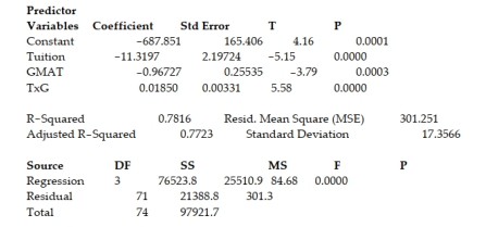Cases Included 75 Missing Cases 0 One of the $t$ -test test statistics is shown on the printout to be the value $t = 5$ . 58 . Interpret this value. A) There is sufficient evidence, at $\alpha = 0.05$ , to indicate that at least one of the variables proposed in the interaction model is useful at predicting the average starting salary of graduates of MBA programs. B) There is insufficient evidence, at $\alpha = 0.05$ , to indicate that at least one of the variables proposed in the interaction model is useful at predicting the average starting salary of graduates of MBA programs. C) There is sufficient evidence, at $\alpha = 0.05$ , to indicate that the interaction between average tuition and average GMAT score is a useful predictor of the average starting salary of graduates of MBA programs. D) There is insufficient evidence, at $\alpha = 0.05$ , to indicate that the interaction between average tuition and average GMAT score is a useful predictor of the average starting salary of graduates of MBA programs.

The table below shows data for n = 20 observations. 1 2 18 3 8 23 5 10 15 2 7 31 6 12 24 4 9 28 5 11 17 2 7 19 3 8 30 7 10 28 5 8 14 3 6 32 7 11 17 2 8 24 5 10 26 6 11 27 6 11 21 3 6 31 7 13 19 2 8 25 5 10 a. Use a first-order regression model to find a least squares prediction equation for the model. b. Find a $95 \%$ confidence interval for the coefficient of $x _ { 1 }$ in your model. Interpret the result. c. Find a $95 \%$ confidence interval for the coefficient of $x _ { 2 }$ in your model. Interpret the result. d. Find $R ^ { 2 }$ and $R _ { a ^ { 2 } } ^ { 2 }$ and interpret these values. e. Test the null hypothesis $H _ { 0 } : \beta _ { 1 } = \beta _ { 2 } = 0$ against the alternative hypothesis $H _ { \mathrm { a } }$ : at least one $\beta _ { i } \neq 0$ . Use $\alpha = .05$ . Interpret the restilt.

Retail price data for n = 60 hard disk drives were recently reported in a computer magazine. Three variables were recorded for each hard disk drive: $y =$ Retail PRICE (measured in dollars) $x _ { 1 } =$ Microprocessor SPEED (measured in megahertz) (Values in sample range from 10 to 40 ) $x _ { 2 } =$ CHIP size (measured in computer processing units) (Values in sample range from 286 to 486 ) a first-order regression model was fit to the data. Part of the printout follows: Dep Var Predict Std Err Lower 95\% Upper 95\% OBS SPEED CHIP PRICE Value Predict Predict Predict Residual 1 33 286 5099.0 4464.9 260.768 3942.7 4987.1 634.1 Interpret the interval given in the printout.

During its manufacture, a product is subjected to four different tests in sequential order. An efficiency expert claims that the fourth (and last) test is unnecessary since its results can be predicted based on the first three tests. To test this claim, multiple regression will be used to model Test4 score $( y )$ , as a function of Test1 score $\left( x _ { 1 } \right)$ , Test 2 score $\left( x _ { 2 } \right)$ , and Test3 score $\left( x _ { 3 } \right)$ . [Note: All test scores range from 200 to 800 , with higher scores indicative of a higher quality product.] Consider the model: $E ( y ) = \beta _ { 1 } + \beta _ { 1 } x _ { 1 } + \beta _ { 2 } x _ { 2 } + \beta _ { 3 } x _ { 3 }$ The first-order model was fit to the data for each of 12 units sampled from the production line. The results are summarized in the printout. SOURCE DF SS $\quad$ MS $\quad$ FVALUE $\quad$ PROB $>$ F Suppose the $95 \%$ confidence interval for $\beta _ { 3 }$ is $( .15 , .47 )$ . Which of the following statements is incorrect? A) At $\alpha = .05$ , there is insufficient evidence to reject $H _ { 0 } : \beta _ { 3 } = 0$ in favor of $H _ { a } : \beta _ { 3 } \neq 0$ . B) We are $95 \%$ confident that the increase in Test 4 score for every 1 -point increase in Test3 score falls between 15 and $.47$ , holding Test1 and Test 2 fixed. C) We are $95 \%$ confident that the Test 3 is a useful linear predictor of Test 4 score, holding Test1 and Test 2 fixed. D) We are $95 \%$ confident that the estimated slope for the Test4-Test 3 line falls between. 15 and .47 holding Test 1 and Test 2 fixed.

When testing the utility of the quadratic model $E ( y ) = \beta _ { 0 } + \beta _ { 1 } x + \beta _ { 2 } x ^ { 2 }$ , the most important tests involve the null hypotheses $H _ { 0 } : \beta 0 = 0$ and $H _ { 0 } : \beta _ { 1 } = 0$ .

One of three surfaces is produced by a complete second-order model with two quantitative independent variables: a paraboloid that opens upward, a paraboloid that opens downward, or a saddle -shaped surface.

A study of the top MBA programs attempted to predict the average starting salary (in $1000's) of graduates of the program based on the amount of tuition (in $1000's) charged by the program and the average GMAT score of the program's students. The results of a regression analysis based on a sample of 75 MBA programs is shown below: Least Squares Linear Regression of Salary 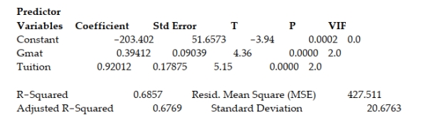Interpret the coefficient for the tuition variable shown on the printout.

A statistics professor gave three quizzes leading up to the first test in his class. The quiz grades and test grade for each of eight students are given in the table. Student Test Grade Quiz 1 Quiz 2 Quiz 3 1 75 8 9 5 2 89 10 7 6 3 73 9 8 7 4 91 8 7 10 5 64 9 6 6 6 78 8 7 6 7 83 10 8 7 8 71 9 4 6 The professor would like to use the data to find a first-order model that he might use to predict a student's grade on the first test using that student's grades on the first three quizzes. a. Identify the dependent and independent variables for the model. b. What is the least squares prediction equation? c. Find the SSE and the estimator of σ2 for the model. 2 Find and Interpret Sample Estimates for β Parameters

For any given model fit to a data set, the sum of the residuals is 0.