Exam 12: Multiple Regression and Model Building
Exam 1: Statistics, Data, and Statistical Thinking73 Questions
Exam 2: Methods for Describing Sets of Data194 Questions
Exam 3: Probability283 Questions
Exam 4: Discrete Random Variables133 Questions
Exam 5: Continuous Random Variables139 Questions
Exam 6: Sampling Distributions47 Questions
Exam 7: Inferences Based on a Single Sample: Estimation With Confidence Intervals124 Questions
Exam 8: Inferences Based on a Single Sample: Tests of Hypothesis140 Questions
Exam 9: Inferences Based on a Two Samples: Confidence Intervals and Tests of Hypotheses94 Questions
Exam 10: Analysis of Variance: Comparing More Than Two Means90 Questions
Exam 11: Simple Linear Regression111 Questions
Exam 12: Multiple Regression and Model Building131 Questions
Exam 13: Categorical Data Analysis60 Questions
Exam 14: Nonparametric Statistics90 Questions
Select questions type
In an interaction model, the relationship between and is linear for each fixed value of but the slopes of the lines relating and may be different for two different fixed values of .
(True/False)
5.0/5  (28)
(28)
A college admissions officer proposes to use regression to model a student's college GPA at graduation in terms of the following two variables: = high school GPA = SAT score
The admissions officer believes the relationship between college GPA and high school GPA is linear and the relationship between SAT score and college GPA is linear. She also believes that the relationship between college GPA and high school GPA depends on the student's SAT score. She proposes the regression model:
Explain how to determine if the relationship between college GPA and SAT score depends on the high school GPA.
(Essay)
4.8/5 (37)
A term that contains the value of a quantitative variable raised to the second power is called a higher -order term.
(True/False)
4.8/5 (36)
Consider the data given in the table below. 1 7 2 6 2 5 3 5 3 4 4 4 4 3 4 2 5 4 5 5 6 6 Plot the data on a scattergram. Does a second-order model seem to be a good fit for the data? Explain.
(Essay)
4.9/5 (32)
An elections officer wants to model voter turnout (y) in a precinct as a function of the type of precinct. Consider the model relating mean voter turnout, E(y), to precinct type: , where if urban, 0 if not
if suburban, 0 if not
(Base level rural)
The -value for the test is .14. Interpret the restll.
A) Do not reject at ; there is no evidence of a difference between the mean voter turnouts for urban, suburban, and rural precincts.
B) Reject at ; the model is useful for predicting voter turnout.
C) Reject at ; there is evidence of a difference between the mean voter turnouts for urban, suburban, and rural precincts.
D) Reject the model since it only explains of the variation.
(Short Answer)
4.8/5 (34)
For a multiple regression model, we assume that the mean of the probability distribution of the random error is 0.
(True/False)
4.8/5 (35)
In any production process in which one or more workers are engaged in a variety of tasks, the total time spent in production varies as a function of the size of the workpool and the level of output of the various activities. In a large metropolitan department store, it is believed that the number of man-hours worked (y) per day by the clerical staff depends on the number of pieces of mail processed per day (x1) and the number of checks cashed per day (x2). Data collected for n = 20 working days were used to fit the model:
A partial printout for the analysis follows:
SOURCE DF SS MS F VALUE PROB > F MODEL 2 7089.06512 3544.53256 13.267 0.0003 ERROR 17 4541.72142 267.16008 C TOTAL 19 11630.78654
ROOT MSE 16.34503 R-SQUARE 0.6095 DEP MEAN 93.92682 ADJ R-SQ 0.5636 C.V. 17.40188
Test to determine if the model is adequate for predicting the number of man-hours worked. Use .
(Essay)
5.0/5 (34)
A study of the top MBA programs attempted to predict the average starting salary (in $1000's) of graduates of the program based on the amount of tuition (in $1000's) charged by the program and the average GMAT score of the program's students. The results of a regression analysis based on a sample of 75 MBA programs is shown below: Least Squares Linear Regression of Salary 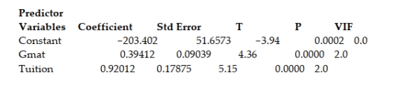 The model was then used to create 95% confidence and prediction intervals for y and for E(Y) when the tuition charged by the MBA program was $75,000 and the GMAT score was 675. The results are shown here: 95% confidence interval for E(Y): ($126,610, $136,640) 95% prediction interval for Y: ($90,113, $173,160) Which of the following interpretations is correct if you want to use the model to estimate Y for a single MBA program?
(Multiple Choice)
4.8/5 (40)
It is safe to conduct t-tests on the individual β parameters in a first-order linear model in order to determine which independent variables are useful for predicting y and which are not.
(True/False)
4.7/5 (29)
When modeling E(y) with a single qualitative independent variable, the number of 0-1 dummy variables in the model is equal to the number of levels of the qualitative variable.
(True/False)
4.8/5 (38)
In any production process in which one or more workers are engaged in a variety of tasks, the total time spent in production varies as a function of the size of the workpool and the level of output of the various activities. In a large metropolitan department store, it is believed that the number of man-hours worked (y) per day by the clerical staff depends on the number of pieces of mail processed per day (x1) and the number of checks cashed per day (x2). Data collected for n = 20 working days were used to fit the model:
A printout for the analysis follows:
SOURCE DF SS MS FVALUE PROB >F
MODEL 2 7089.06512 3544.53256 13.267 0.0003 ERROR 17 4541.72142 267.16008 C TOTAL 19 11630.78654
PARAMETER STANDARD TFOR 0: VARIABLE DF ESTIMATE ERROR PARAMETER =0 PROB >|T|
INTERCEPT 1 114.420972 18.68485744 6.124 0.0001 X1 1 -0.007102 0.00171375 -4.144 0.0007 X2 1 0.037290 0.02043937 1.824 0.0857
Actual Predict Lower 95 \% CL Upper 95 \% CL OBS X1 X2 Value Value Residual Predict Predict 1 7781 644 74.707 83.175 -8.468 47.224 119.126
Test to determine if there is a positive linear relationship between the number of man-hours worked, , and the number of checks cashed per day, . Use .
(Essay)
4.8/5 (29)
The rejection of the null hypothesis in a global F-test means that the model is the best model for providing reliable estimates and predictions.
(True/False)
4.7/5 (41)
The confidence interval for the mean E(y) is narrower that the prediction interval for y.
(True/False)
4.7/5 (33)
A study of the top MBA programs attempted to predict the average starting salary (in $1000's) of graduates of the program based on the amount of tuition (in $1000's) charged by the program and the average GMAT score of the program's students. The results of a regression analysis based on a sample of 75 MBA programs is shown below: Least Squares Linear Regression of Salary 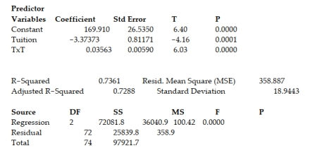 Cases Included 75 Missing Cases 0
One of the -test test statistics is shown on the printout to be the value . Interpret this value.
A) There is insufficient evidence, at , to indicate that at least one of the variables proposed in the interaction model is useful at predicting the average starting salary of graduates of MBA programs.
B) There is sufficient evidence, at , to indicate that at least one of the variables proposed in the interaction model is useful at predicting the average starting salary of graduates of MBA programs.
C) There is sufficient evidence, at , to indicate that there is a curvilinear relationship between average starting salary of graduates of MBA programs and the tuition of the MBA program.
D) There is sufficient evidence, at , to indicate that there is a linear relationship between average starting salary of graduates of MBA programs and the tuition of the MBA program.
Cases Included 75 Missing Cases 0
One of the -test test statistics is shown on the printout to be the value . Interpret this value.
A) There is insufficient evidence, at , to indicate that at least one of the variables proposed in the interaction model is useful at predicting the average starting salary of graduates of MBA programs.
B) There is sufficient evidence, at , to indicate that at least one of the variables proposed in the interaction model is useful at predicting the average starting salary of graduates of MBA programs.
C) There is sufficient evidence, at , to indicate that there is a curvilinear relationship between average starting salary of graduates of MBA programs and the tuition of the MBA program.
D) There is sufficient evidence, at , to indicate that there is a linear relationship between average starting salary of graduates of MBA programs and the tuition of the MBA program.
(Short Answer)
4.8/5 (27)
A study of the top MBA programs attempted to predict the average starting salary (in $1000's) of graduates of the program based on the amount of tuition (in $1000's) charged by the program and the average GMAT score of the program's students. The results of a regression analysis based on a sample of 75 MBA programs is shown below: Least Squares Linear Regression of Salary 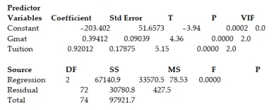 Interpret the -value for the global -test shown on the printout.
A) At , there is insufficient evidence to indicate that something in the regression model is useful for predicting the average starting salary of the graduates of an MBA program.
B) At , there is insufficient evidence to indicate that the average GMAT score of the MBA program's students is useful for predicting the average starting salary of the graduates of an MBA program.
C) At , there is stufficient evidence to indicate that the average GMAT score of the MBA program's students is useful for predicting the average starting salary of the graduates of an MBA program.
D) At , there is sufficient evidence to indicate that something in the regression model is useful for predicting the average starting salary of the graduates of an MBA program.
Interpret the -value for the global -test shown on the printout.
A) At , there is insufficient evidence to indicate that something in the regression model is useful for predicting the average starting salary of the graduates of an MBA program.
B) At , there is insufficient evidence to indicate that the average GMAT score of the MBA program's students is useful for predicting the average starting salary of the graduates of an MBA program.
C) At , there is stufficient evidence to indicate that the average GMAT score of the MBA program's students is useful for predicting the average starting salary of the graduates of an MBA program.
D) At , there is sufficient evidence to indicate that something in the regression model is useful for predicting the average starting salary of the graduates of an MBA program.
(Short Answer)
4.8/5 (36)
An elections officer wants to model voter turnout (y) in a precinct as a function of the type of precinct. Consider the model relating mean voter turnout, E(y), to precinct type: E(y)=++ , where =1 if urban, 0 if not =1 if suburban, 0 if not (Base level = rural)
Interpret the value of .
A) the mean voter turnout for rural precincts
B) the -intercept of the line
C) the difference between the mean voter turnout for urban and rural precincts
D) the mean voter turnout for urban precincts
(Short Answer)
4.8/5 (28)
Retail price data for n = 60 hard disk drives were recently reported in a computer magazine. Three variables were recorded for each hard disk drive: Retail PRICE (measured in dollars)
Microprocessor SPEED (measured in megahertz)
(Values in sample range from 10 to 40 )
CHIP size (measured in computer processing units)
(Values in sample range from 286 to 486)
A first-order regression model. was fit to the data. Part of the printout follows:
INTERCEPT 1 -373.526392 1258.1243396 -0.297 0.7676 SPEED 1 104.838940 22.36298195 4.688 0.0001 CHIP 1 3.571850 3.89422935 0.917 0.3629
Identify and interpret the estimate of .
(Essay)
4.8/5 (26)
A statistics professor gave three quizzes leading up to the first test in his class. The quiz grades and test grade for each of eight students are given in the table. Student Test Grade Quiz 1 Quiz 2 Quiz 3 1 75 8 9 5 2 89 10 7 6 3 73 9 8 7 4 91 8 7 10 5 64 9 6 6 6 78 8 7 6 7 83 10 8 7 8 71 9 4 6 The professor fit a first-order model to the data that he intends to use to predict a student's grade on the first test using that student's grades on the first three quizzes. Test the null hypothesis against the alternative hypothesis : at least one . Use . Interpret the result. α = .05. Interpret the result. 12.4 Using the Model for Estimation and Prediction 1 Find and Interpret Prediction Interval
(Essay)
4.8/5 (38)
In any production process in which one or more workers are engaged in a variety of tasks, the total time spent in production varies as a function of the size of the workpool and the level of output of the various activities. In a large metropolitan department store, it is believed that the number of man-hours worked (y) per day by the clerical staff depends on the number of pieces of mail processed per day (x1) and the number of checks cashed per day (x2). Data collected for n = 20 working days were used to fit the model:
A partial printout for the analysis follows:
Actual Predict Lower 95\% CL Upper 95\% CL OBS X1 X2 Value Value Residual Predict Predict 1 7781 644 74.707 83.175 -8.468 47.224 119.126 Interpret the 95% prediction interval for y shown on the printout.
(Multiple Choice)
4.8/5 (38)
Filters
- Essay(0)
- Multiple Choice(0)
- Short Answer(0)
- True False(0)
- Matching(0)