Exam 12: Multiple Regression and Model Building

In the quadratic model $E ( y ) = \beta _ { 0 } + \beta _ { 1 } x + \beta _ { 2 } x ^ { 2 } , \text { a negative value of } \beta _ { 1 }$ indicates downward concavity.

A fast food chain test marketing a new sandwich chose 18 of its stores in one major metropolitan area. Nine of the stores were in malls and nine were free standing. The sandwich was offered at three different introductory prices. The table shows the number of new sandwiches sold at each location for each location type and price combination. 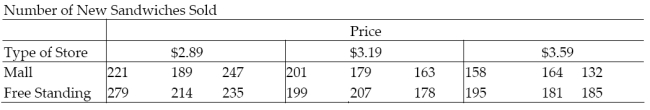a. Write a model for the mean number of sandwiches sold, E(y), assuming that the relationship between E(y) and price, x1, is first-order. b. Fit the model to the data. c. Write the prediction equations for mall and free-standing stores. d. Do the data provide sufficient evidence that the change in number of sandwiches sold with respect to price is different for mall and free-standing stores? Use α = .01. 12.9 Comparing Nested Models (Optional) 1 Conduct Test to Compare Complete and Reduced Models

In the presence of multicollinearity, the predicted values of $\hat{y}$ are actually quite good for values of x far outside the range of the sampled values of x.

A study of the top MBA programs attempted to predict the average starting salary (in $1000's) of graduates of the program based on the amount of tuition (in $1000's) charged by the program and the average GMAT score of the program's students. The results of a regression analysis based on a sample of 75 MBA programs is shown below: Least Squares Linear Regression of Salary 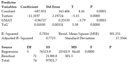Cases Included 75 Missing Cases 0 The global-f test statistic is shown on the printout to be the value $\mathrm { F } = 84.68$ . Interpret this value. A) There is sufficient evidence, at $\alpha = 0.05$ , to indicate that at least one of the variables proposed in the interaction model is useful at predicting the average starting salary of graduates of MBA programs. B) There is instufficient evidence, at $\alpha = 0.05$ , to indicate that at least one of the variables proposed in the interaction model is useful at predicting the average starting salary of graduates of MBA programs. C) There is sufficient evidence, at $\alpha = 0.05$ , to indicate that the interaction between average tuition and average GMAT score is a useful predictor of the average starting salary of graduates of MBA programs. D) There is insufficient evidence, at $\alpha = 0.05$ , to indicate that the interaction between average tuition and average GMAT score is a useful predictor of the average starting salary of graduates of MBA programs.

It is desired to build a regression model to predict $y =$ the sales price of a single family home, based on the $x _ { 1 } =$ size of the hotise and $x _ { 2 } =$ the neighborhood the home is located in. The goal is to compare the prices of homes that are located in two different neighborhoods. The following complete 2 nd-order model is proposed: E(y) = $\beta _ { 0 } + \beta _ { 1 } x _ { 1 } + \beta _ { 2 } x _ { 1 } ^ { 2 } + \beta _ { 3 } x _ { 2 } + \beta _ { 4 } x _ { 1 } x _ { 2 } + \beta _ { 5 } x _ { 1 } ^ { 2 } x _ { 2 }$ . What hypothesis should be tested to determine if the quadratic terms are necessary to predict the sales price of a home? A) $\mathrm { H } _ { 0 } : \beta _ { 1 } = \beta _ { 2 } = \beta _ { 3 } = \beta _ { 4 } = \beta _ { 5 } = 0$ B) $\mathrm { H } _ { 0 } : \beta _ { 2 } = \beta _ { 5 } = 0$ C) $\mathrm { H } _ { 0 } : \beta _ { 1 } = \beta _ { 3 } = \beta _ { 4 } = 0$ D) $\mathrm { H } _ { 0 } : \beta _ { 1 } = \beta _ { 2 } = \beta _ { 3 } = 0$

In any production process in which one or more workers are engaged in a variety of tasks, the total time spent in production varies as a function of the size of the workpool and the level of output of the various activities. In a large metropolitan department store, it is believed that the number of man-hours worked $( y )$ per day by the clerical staff depends on the number of pieces of mail processed per day $\left( x _ { 1 } \right)$ and the number of checks cashed per day $\left( x _ { 2 } \right)$ . Data collected for $n = 20$ working days were used to fit the model: $E ( y ) = \beta _ { 0 } + \beta _ { 1 } x _ { 1 } + \beta _ { 2 } x _ { 2 }$ A partial printout for the analysis follows: Parameter Estimates PARAMETER STANDARD T FOR 0: VARIABLE DF ESTIMATE T FRROR PARAMETER = 0 PROB >|T| INTERCEPT 1 114.420972 18.6848744 6.124 0.0001 X1 1 -0.007102 0.00171375 -4.144 0.0007 X2 1 0.037290 0.02043937 1.824 0.0857 Calculate a $95 \%$ confidence interval for $\beta _ { 1 }$ . A) $- .007 \pm .0036$ B) $- .007 \pm .0017$ C) $- .007 \pm .0007$ D) $- 4.144 \pm .0007$

The printout shows the results of a first-order regression analysis relating the sales price y of a product to the time in hours x1 and the cost of raw materials x2 needed to make the product. SUMMARY OUTPUT Regression Statistics Multiple R 0.997578302 R Square 0.995162468 Adjusted R Square 0.990324936 Standard Error 1.185250723 Observations 5 ANOVA df SS MS F Significance F Regression 2 577.9903614 288.9952 205.717 0.004837532 Residual 2 2.809638554 1.404819 Total 4 580.8 Coefficients Standard Error tStat P-value Lower 95\% Upper 95\% Intercept -26.48433735 3.674668773 -7.20727 0.018713 -42.29517198 -10.67350271 Time -2.168674699 4.11406532 -0.52714 0.650732 -19.8700814 15.532732 Materials 8.142168675 1.094681583 7.437933 0.0176 3.432130693 12.85220666 a. What is the least squares prediction equation? b. Identify the SSE from the printout. c. Find the estimator of σ2 for the model.

Consider the partial printout below. Coefficients Standard Error t Stat P-value Lower 95\% Upper 95\% Intercept -63.14873931 25.09115112 -2.516773304 0.045484943 -124.5446192 -1.752859365 14.72507864 8.113581741 1.814867849 0.119466699 -5.128155197 34.57831248 X2 12.48784546 4.686063743 2.664890224 0.037279879 1.021452165 23.95423875 X1X2 -1.886935135 1.344999834 -1.402925924 0.210210141 -5.178033575 1.404163305 Is there evidence (at α = .05) that x1 and x2 interact? Explain. 12.6 Quadratic and Other Higher Order Models 1 Write and Interpret Second-Order Model

Consider the interaction model $E ( y ) = 7 + 3 x _ { 1 } - 4 x _ { 2 } + 5 x _ { 1 } x _ { 2 }$ . Find the slope of the line relating $E ( y )$ and $x _ { 1 }$ when $x _ { 2 } = 2$ when x2 = 2.

One advantage to writing a single model that includes all levels of a qualitative variable rather a separate model for each level is that we obtain a pooled estimate of $\sigma ^ { 2 }$ .

During its manufacture, a product is subjected to four different tests in sequential order. An efficiency expert claims that the fourth (and last) test is unnecessary since its results can be predicted based on the first three tests. To test this claim, multiple regression will be used to model Test4 score (y), as a function of Test1 score (x1), Test 2 score (x2), and Test3 score (x3). [Note: All test scores range from 200 to 800, with higher scores indicative of a higher quality product.] Consider the model: $E ( y ) = \beta _ { 1 } + \beta _ { 1 } x _ { 1 } + \beta _ { 2 } x _ { 2 } + \beta _ { 3 } x _ { 3 }$ The first-order model was fit to the data for each of 12 units sampled from the production line. A 95% prediction interval for Test4 score of a product with Test1 = 590, Test2 = 750, and Test3 = 710 is (583, 793). Interpret this result.