Exam 11: Simple Linear Regression
Exam 1: Statistics, Data, and Statistical Thinking77 Questions
Exam 2: Methods for Describing Sets of Data187 Questions
Exam 3: Probability284 Questions
Exam 4: Discrete Random Variables134 Questions
Exam 5: Continuous Random Variables138 Questions
Exam 6: Sampling Distributions52 Questions
Exam 7: Inferences Based on a Single Sample: Estimation With Confidence Intervals125 Questions
Exam 8: Inferences Based on a Single144 Questions
Exam 9: Inferences Based on Two Samples: Confidence Intervals and Tests of Hypotheses100 Questions
Exam 10: Analysis of Variance: Comparing More Than Two Means91 Questions
Exam 11: Simple Linear Regression113 Questions
Exam 12: Multiple Regression and Model Building131 Questions
Exam 13: Categorical Data Analysis60 Questions
Exam 14: Nonparametric Statistics Available Online87 Questions
Select questions type
Consider the following pairs of observations: x 2 3 5 5 6 y 1.3 1.6 2.1 2.2 2.7 Find and interpret the value of the coefficient of correlation.
Free
(Essay)
4.8/5  (32)
(32)
Correct Answer: Verified
There is a strong linear relationship between and .
Consider the following pairs of observations: x 2 3 5 5 6 y 1.3 1.6 2.1 2.2 2.7 Find and interpret the value of the coefficient of determination.
Free
(Essay)
4.9/5 (36)
Correct Answer:Verified
of the sample variation in values can be attributed to the linear relationship between and .
A realtor collected the following data for a random sample of ten homes that recently sold
in her area. House Asking Price Days on Market \ 114,500 29 \ 149,900 16 \ 154,700 59 \ 159,900 42 \ 160,000 72 \ 165,900 45 \ 169,700 12 \ 171,900 39 \ 175,000 81 \ 289,900 121 a. Construct a scattergram for the data.
b. Find the least squares line for the data and plot the line on your scattergram.
c. Test whether the number of days on the market, y, is positively linearly related to the
Free
(Essay)
4.8/5 (27)
Correct Answer:Verified
a.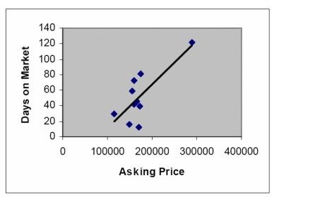
b. ;
c. The test statistic is .
Based on 8 degrees of freedom, the rejection region is . Since the test statistic falls in the rejection region, we reject the null hypothesis and conclude that the number of days on the market, , is positively linearly related to the asking price, .
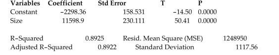
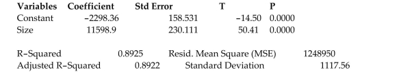
A study of the top 75 MBA programs attempted to predict the average starting salary (in $1000's) of graduates of the program based on the amount of tuition (in $1000's)charged by the program.
The results of a simple linear regression analysis are shown below: Least Squares Linear Regression of Salary
Predictor
Variables Coefficient Std Error T P Constant 18.1849 10.3336 1.76 0.0826 Size 1.47494 0.14017 10.52 0.0000
 In addition, we are told that the coefficient of correlation was calculated to be . Interpret this result.
(Multiple Choice)
4.9/5 (29)
State the four basic assumptions about the general form of the probability distribution of
the random error ε.
(Essay)
4.9/5 (37)
The dean of the Business School at a small Florida college wishes to determine whether the grade-point average (GPA)of a graduating student can be used to predict the graduateʹs starting
Salary. More specifically, the dean wants to know whether higher GPAs lead to higher starting
Salaries. Records for 23 of last yearʹs Business School graduates are selected at random, and data
On GPA (x)and starting salary (y, in $thousands)for each graduate were used to fit the model
The results of the simple linear regression are provided below.
=4.25+2.75x, S=5.15,S=1.87 SSyy=15.17,SSE=1.0075
Calculate the value of , the coefficient of determination.
(Multiple Choice)
4.8/5 (32)
For the situation above, give a practical interpretation of .
(Multiple Choice)
4.8/5 (29)
For the situation above, give a practical interpretation of .
(Multiple Choice)
4.8/5 (33)
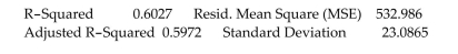
What is the relationship between diamond price and carat size? 307 diamonds were sampled and a straight-line relationship was hypothesized between y = diamond price (in dollars)and x = size of
The diamond (in carats). The simple linear regression for the analysis is shown below: Least Squares Linear Regression of PRICE
Predictor
 Interpret the standard deviation of the regression model.
(Multiple Choice)
4.9/5 (37)
What is the relationship between diamond price and carat size? 307 diamonds were sampled and a straight-line relationship was hypothesized between y = diamond price (in dollars)and x = size of
The diamond (in carats). The simple linear regression for the analysis is shown below: Least Squares Linear Regression of PRICE
Predictor
 Interpret the coefficient of determination for the regression model.
(Multiple Choice)
4.9/5 (35)
A county real estate appraiser wants to develop a statistical model to predict the appraised value of houses in a section of the county called East Meadow. One of the many variables thought to be
An important predictor of appraised value is the number of rooms in the house. Consequently, the
Appraiser decided to fit the simple linear regression model:
where appraised value of the house (in thousands of dollars) and number of rooms. Using data collected for a sample of houses in East Meadow, the following results were obtained:
Give a practical interpretation of the estimate of the slope of the least squares line.
(Multiple Choice)
4.9/5 (36)
In a study of feeding behavior, zoologists recorded the number of grunts of a warthog
feeding by a lake in the 15 minute period following the addition of food. The data showing
the number of grunts and and the age of the warthog (in days)are listed below: Number of Grunts Age (days) 83 118 61 134 32 148 37 153 56 160 33 167 55 176 10 182 13 188 Find and interpret the value of .
(Essay)
4.8/5 (40)
a. Complete the table. 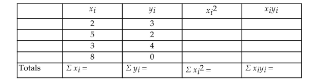 b. Find , and .
c. Write the equation of the least squares line.
b. Find , and .
c. Write the equation of the least squares line.
(Essay)
4.7/5 (41)
A company keeps extensive records on its new salespeople on the premise that sales
should increase with experience. A random sample of seven new salespeople produced
the data on experience and sales shown in the table. Months on Job Monthly Sales y (\ thousands) 2 2.4 4 7.0 8 11.3 12 15.0 1 .8 5 3.7 9 12.0
Summary statistics yield , and . Using , find and interpret the coefficient of determination.
(Essay)
4.7/5 (35)
What is the relationship between diamond price and carat size? 307 diamonds were sampled and a straight-line relationship was hypothesized between y = diamond price (in dollars)and x = size of
The diamond (in carats). The simple linear regression for the analysis is shown below: Least Squares Linear Regression of PRICE
 The model was then used to create confidence and prediction intervals for and for E(Y) when the carat size of the diamond was 1 carat. The results are shown here:
confidence interval for
prediction interval for
Which of the following interpretations is correct if you want to use the model to estimate for all 1 -carat diamonds?
The model was then used to create confidence and prediction intervals for and for E(Y) when the carat size of the diamond was 1 carat. The results are shown here:
confidence interval for
prediction interval for
Which of the following interpretations is correct if you want to use the model to estimate for all 1 -carat diamonds?
(Multiple Choice)
4.8/5 (37)
In team-teaching, two or more teachers lead a class. A researcher tested the use of 74)
team-teaching in mathematics education. Two of the variables measured on each teacher
in a sample of 159 mathematics teachers were years of teaching experience x and reported
success rate y (measured as a percentage)of team-teaching mathematics classes.
The correlation coefficient for the sample data was reported as r = -0.3. Interpret this
result.
(Essay)
4.9/5 (42)
An academic advisor wants to predict the typical starting salary of a graduate at a top business school using the GMAT score of the school as a predictor variable. A simple linear regression of
SALARY versus GMAT using 25 data points is shown below.
Give a practical interpretation of .
(Multiple Choice)
4.9/5 (24)
Is the number of games won by a major league baseball team in a season related to the
teamʹs batting average? Data from 14 teams were collected and the summary statistics
yield: , and
Assume and . Conduct a test of hypothesis to determine if a positive linear relationship exists between team batting average and number of wins. Use .
(Essay)
4.8/5 (32)
Consider the following pairs of observations: x 2 3 5 5 6 y 1.3 1.6 2.1 2.2 2.7
a. Construct a scattergram for the data. Does the scattergram suggest that is positively linearly related to ?
b. Find the slope of the least squares line for the data and test whether the data provide sufficient evidence that is positively linearly related to . Use .
(Essay)
4.7/5 (27)
Filters
- Essay(0)
- Multiple Choice(0)
- Short Answer(0)
- True False(0)
- Matching(0)