Exam 12: Multiple Regression and Model Building

It is desired to build a regression model to predict $\mathrm { y } =$ the sales price of a single family home, based on the $x _ { 1 } =$ size of the house and $x _ { 2 } =$ the neighborhood the home is located in. The goal is to compare the prices of homes that are located in two different neighborhoods. The following complete 2nd-order model is proposed: $\mathrm { E } ( \mathrm { y } ) = \beta _ { 0 } + \beta _ { 1 } \mathrm { x } _ { 1 } + \beta _ { 2 } \mathrm { x } _ { 1 } ^ { 2 } + \beta _ { 3 } \mathrm { x } _ { 2 } + \beta _ { 4 } \mathrm { x } _ { 1 } \mathrm { x } _ { 2 } + \beta _ { 5 } \mathrm { x } _ { 1 } ^ { 2 } \mathrm { x } _ { 2 }$ . What hypothesis should be tested to determine if the quadratic terms are necessary to predict the sales price of a home?

In the quadratic model $E ( y ) = \beta _ { 0 } + \beta _ { 1 } x + \beta _ { 2 } x ^ { 2 }$ , a negative value of $\beta _ { 1 }$ indicates downward concavity.

During its manufacture, a product is subjected to four different tests in sequential order. An efficiency expert claims that the fourth (and last) test is unnecessary since its results can be predicted based on the first three tests. To test this claim, multiple regression will be used to model Test4 score $( y )$ , as a function of Test1 score $\left( x _ { 1 } \right)$ , Test 2 score $\left( x _ { 2 } \right)$ , and Test3 score $\left( x _ { 3 } \right)$ ). [Note: All test scores range from 200 to 800 , with higher scores indicative of a higher quality product.] Consider the model: $E ( y ) = \beta _ { 1 } + \beta _ { 1 } x _ { 1 } + \beta _ { 2 } x _ { 2 } + \beta _ { 3 } x _ { 3 }$ The first-order model was fit to the data for each of 12 units sampled from the production line. The results are summarized in the printout. SOURCE DF SS MS FVALUE PROB >F MODEL 3 151417 50472 18.16 .0075 ERROR 8 22231 2779 TOTAL 12 173648 ROOT MSE 52.72 R-SQUARE 0.872 DEP MEAN 645.8 ADJ R-SQ 0.824 PARAMETER STANDARD T FOR 0: VARIABLE ESTIMATE ERROR PARAMETER =0 PROB >|| INTERCEPT 11.98 80.50 0.15 0.885 X1(TEST1) 0.2745 0.1111 2.47 0.039 X2(TEST2) 0.3762 0.0986 3.82 0.005 X3(TEST3) 0.3265 0.0808 4.04 0.004 Suppose the $95 \%$ confidence interval for $\beta _ { 3 }$ is $( .15 , .47 )$ . Which of the following statements is incorrect?

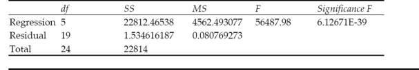
The complete second-order model $E ( y ) = \beta _ { 0 } + \beta _ { 1 } x _ { 1 } + \beta _ { 2 } x _ { 2 } + \beta _ { 3 } x _ { 1 } x _ { 2 } + \beta _ { 4 } x _ { 1 } ^ { 2 } + \beta _ { 5 } x _ { 2 } ^ { 2 }$ was fit to $n = 25$ data points. The printout is shown below. ANOVA 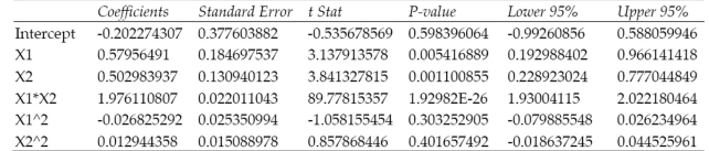a. Write the complete second-order model for the data. b. Is there sufficient evidence to indicate that at least one of the parameters $\beta _ { 1 } , \beta _ { 2 } , \beta _ { 3 } , \beta _ { 4 }$ , and $\beta _ { 5 }$ is nonzero? Test using $\alpha = .05$ . c. Test $H _ { 0 } : \beta _ { 3 } = 0$ against $H _ { \mathrm { a } } : \beta _ { 3 } \neq 0$ . Use $\alpha = .01$ . d. Test $H _ { 0 } : \beta _ { 4 } = 0$ against $H _ { \mathrm { a } } : \beta _ { 4 } \neq 0$ . Use $\alpha = .01$ .

A certain type of rare gem serves as a status symbol for many of its owners. In theory, for low prices, the demand decreases as the price of the gem increases. However, experts hypothesize that when the gem is valued at very high prices, the demand increases with price due to the status the owners believe they gain by obtaining the gem. Thus, the model proposed to best explain the demand for the gem by its price is the quadratic model $E ( y ) = \beta _ { 0 } + \beta _ { 1 } x + \beta _ { 2 } x ^ { 2 }$ where y = Demand (in thousands)and x = Retail price per carat (dollars). This model was fit to data collected for a sample of 12 rare gems. A portion of the printout is given below: SOURCE DF SS MS F PR > Model 2 115145 57573 373 .0001 Error 9 1388 154 TOTAL 11 116533 Root MSE 12.42 R-Square .988 PARAMETER T for HO: VARIABLES ESTIMATES STD. ERROR PARAMETER =0 PR >|| INTERPCEP 286.42 9.66 29.64 .0001 X -.31 .06 -5.14 .0006 X.X .000067 .00007 .95 .3647 Does the quadratic term contribute useful information for predicting the demand for the gem? Use $\alpha = .10$ .

As part of a study at a large university, data were collected on n = 224 freshmen computer science (CS)majors in a particular year. The researchers were interested in modeling y, a studentʹs grade point average (GPA)after three semesters, as a function of the following independent variables (recorded at the time the students enrolled in the university): $x _ { 1 } =$ average high school grade in mathematics (HSM) $x _ { 2 } =$ average high school grade in science (HSS) $x _ { 3 } =$ average high school grade in English (HSE) $x _ { 4 } =$ SAT mathematics score (SATM) $x _ { 5 } =$ SAT verbal score (SATV) A first-order model was fit to data with $R _ { a } ^ { 2 } = .193$ . Interpret the value of the adjusted coefficient of determination $R _ { a } ^ { 2 }$ .

In any production process in which one or more workers are engaged in a variety of tasks, the total time spent in production varies as a function of the size of the workpool and the level of output of the various activities. In a large metropolitan department store, it is believed that the number of man-hours worked $( y )$ per day by the clerical staff depends on the number of pieces of mail processed per day $\left( x _ { 1 } \right)$ and the number of checks cashed per day $\left( x _ { 2 } \right)$ . Data collected for $n = 20$ working days were used to fit the model: $E ( y ) = \beta _ { 0 } + \beta _ { 1 } x _ { 1 } + \beta _ { 2 } x _ { 2 }$ A partial printout for the analysis follows: 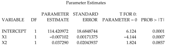Calculate a $95 \%$ confidence interval for $\beta _ { 1 }$ .

An elections officer wants to model voter turnout (y)in a precinct as a function of the type of precinct. Consider the model relating mean voter turnout, $E ( y )$ , to precinct type: E(y)=++, where =1 if urban, 0 if not =1 if suburban, 0 if not (Base level = rural) Interpret the value of $\beta _ { 2 }$ .

For a multiple regression model, we assume that the mean of the probability distribution of the random error is 0.

During its manufacture, a product is subjected to four different tests in sequential order. An efficiency expert claims that the fourth (and last) test is unnecessary since its results can be predicted based on the first three tests. To test this claim, multiple regression will be used to model Test4 score (y), as a function of Test1 score $\left( x _ { 1 } \right)$ , Test 2 score $\left( x _ { 2 } \right)$ , and Test3 score ( $\left. x _ { 3 } \right)$ ). [Note: All test scores range from 200 to 800 , with higher scores indicative of a higher quality product.] Consider the model: $E ( y ) = \beta _ { 1 } + \beta _ { 1 } x _ { 1 } + \beta _ { 2 } x _ { 2 } + \beta _ { 3 } x _ { 3 }$ The first-order model was fit to the data for each of 12 units sampled from the production line. The results are summarized in the printout. SOURCE DF SS MS F VALUE PROB > F MODEL 3 151417 50472 18.16 .0075 ERROR 8 22231 2779 TOTAL 12 173648 ROOT MSE 52.72 R-SQUARE 0.872 DEP MEAN 645.8 ADJ R-SQ 0.824 PARAMETER STANDARD T FOR 0: VARIABLE ESTIMATE ERROR PARAMETER =0 PROB >|| INTERCEPT 11.98 80.50 0.15 0.885 X1(TEST1) 0.2745 0.1111 2.47 0.039 X2(TEST2) 0.3762 0.0986 3.82 0.005 X3(TEST3) 0.3265 0.0808 4.04 0.004 Compute a $95 \%$ confidence interval for $\beta _ { 3 }$ .

In regression, it is desired to predict the dependent variable based on values of other related independent variables. Occasionally, there are relationships that exist between the independent Variables. Which of the following multiple regression pitfalls does this example describe?

The printout shows the results of a first-order regression analysis relating the sales price $y$ of a product to the time in hours $x _ { 1 }$ and the cost of raw materials $x _ { 2 }$ needed to make the product. SUMMARY OUTPUT Regression Statistics Multiple R 0.997578302 R Square 0.995162468 Adjusted R Square 0.990324936 Standard Error 1.185250723 Observations 5 ANOVA df SS MS F Significance F Regression 2 577.9903614 288.9952 205.717 0.004837532 Residual 2 2.809638554 1.404819 Total 4 580.8 Coefficients Standard Error t Stat P-value Lower 95\% Upper 95\% Intercept -26.48433735 3.674668773 -7.20727 0.018713 -42.29517198 -10.67350271 Time -2.168674699 4.11406532 -0.52714 0.650732 -19.8700814 15.532732 12.85220666 Materials 8.142168675 1.094681583 7.437933 0.0176 3.432130693 12.05 a. What is the least squares prediction equation? b. Identify the SSE from the printout. c. Find the estimator of $\sigma ^ { 2 }$ for the model.

We decide to conduct a multiple regression analysis to predict the attendance at a major league baseball game. We use the size of the stadium as a quantitative independent variable and the type Of game as a qualitative variable (with two levels - day game or night game). We hypothesize the Following model: $\mathrm { E } ( \mathrm { y } ) = \beta _ { 0 } + \beta _ { 1 } \mathrm { x } _ { 1 } + \beta _ { 2 } \mathrm { x } _ { 2 } + \beta _ { 3 } \mathrm { x } _ { 3 }$ Where $\mathrm { x } _ { 1 } =$ size of the stadium $x _ { 2 } = 1$ if a day game, 0 if a night game A plot of the $y - x$ relationship would show:

Retail price data for n = 60 hard disk drives were recently reported in a computer magazine. Three variables were recorded for each hard disk drive: $y =$ Retail PRICE (measured in dollars) $x _ { 1 } =$ Microprocessor SPEED (measured in megahertz) (Values in sample range from 10 to 40 ) $x _ { 2 } =$ CHIP size (measured in computer processing units) (Values in sample range from 286 to 486 ) A first-order regression model was fit to the data. Part of the printout follows: 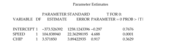Identify and interpret the estimate for the SPEED $\beta$ -coefficient, $\hat { \beta } _ { 1 }$ .

A nested model F-test can only be used to determine whether second-order terms should be included in the model.

Consider the model $y = \beta _ { 0 } + \beta _ { 1 } x _ { 1 } + \beta _ { 2 } x _ { 2 } + \beta _ { 3 } x _ { 3 } + \varepsilon$ where $x _ { 1 }$ is a quantitative variable and $x _ { 2 }$ and $x _ { 3 }$ are dummy variables describing a qualitative variable at three levels using the coding scheme $x _ { 2 } = \left\{ \begin{array} { l l } 1 & \text { if level } 2 \\ 0 & \text { otherwise } \end{array} \quad x _ { 3 } = \left\{ \begin{array} { l l } 1 & \text { if level } 3 \\ 0 & \text { otherwise } \end{array} \right. \right.$ The resulting least squares prediction equation is $\hat { y } = 16.3 + 2.3 x _ { 1 } + 3.5 x _ { 2 } + 18 x _ { 3 }$ . What is the response line (equation) for $E ( y )$ when $x _ { 2 } = 0$ and $x _ { 3 } = 1$ ?

We expect all or almost all of the residuals to fall within 2 standard deviations of 0.

In the first-order model $E ( y ) = \beta _ { 0 } + \beta _ { 1 } x _ { 1 } + \beta _ { 2 } x _ { 2 } + \beta _ { 3 } x _ { 3 } , \beta _ { 2 }$ represents the slope of the line relating $y$ to $x _ { 2 }$ when $\beta _ { 1 }$ and $\beta _ { 3 }$ are both held fixed.

The confidence interval for the mean E(y)is narrower that the prediction interval for y.

One advantage to writing a single model that includes all levels of a qualitative variable rather a separate model for each level is that we obtain a pooled estimate of $\sigma ^ { 2 } .$