Exam 16: Time-Series Forecasting

Microsoft Excel was used to obtain the following quadratic trend equation: Sales = 100 - 10X + 15X². The data used was from 2001 through 2010 coded 0 to 9. The forecast for 2011 is ________.

The method of least squares may be used to estimate both linear and curvilinear trends.

TABLE 16-4 The number of cases of merlot wine sold by a Paso Robles winery in an 8-year period follows. Year Cases of Wine 2003 270 2004 356 2005 398 2006 456 2007 358 2008 500 2009 410 2010 376 -Referring to Table 16-4, exponential smoothing with a weight or smoothing constant of 0.4 will be used to smooth the wine sales. The value of E₅, the smoothed value for 2007 is ________.

TABLE 16-7 The executive vice-president of a drug manufacturing firm believes that the demand for the firm's most popular drug has been evidencing an exponential trend since 1995. She uses Microsoft Excel to obtain the partial output below. The dependent variable is the log base 10 of the demand for the drug, while the independent variable is years, where 1995 is coded as 0, 1996 is coded as 1, etc. SUMMARY OUTPUT Regression Statistics Multiple R 0.996 R Square 0.992 Adjusted R Square 0.991 Standard Error 0.02831 Observations 12 Coefficients Intercept 1.44 Coded Year 0.068 -Referring to Table 16-7, the fitted trend value for 2000 is ________.

TABLE 16-8 The manager of a marketing consulting firm has been examining his company's yearly profits. He believes that these profits have been showing a quadratic trend since 1990. He uses Microsoft Excel to obtain the partial output below. The dependent variable is profit (in thousands of dollars), while the independent variables are coded years and squared of coded years, where 1990 is coded as 0, 1991 is coded as 1, etc. SUMMARY OUTPUT Regression Statistics Multiple R 0.998 R Square 0.996 Adjusted R Square 0.996 Standard Error 4.996 Observations 17 Coefficients Intercept 35.5 Coded Year 0.45 Year Squared 1.00 -Referring to Table 16-8, the forecast for profits in 2015 is ________.

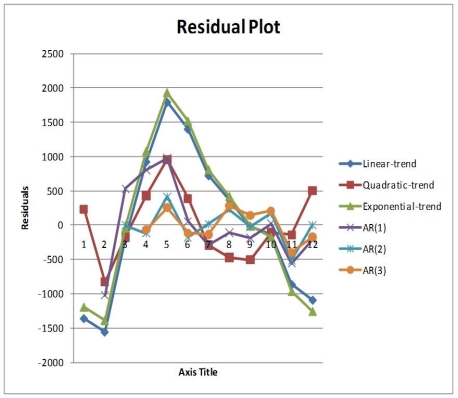
TABLE 16-13 Given below is the monthly time-series data for U.S. retail sales of building materials over a specific year. Month Retail Sales 1 6,594 2 6,610 3 8,174 4 9,513 5 10,595 6 10,415 7 9,949 8 9,810 9 9,637 10 9,732 11 9,214 12 9,201 The results of the linear trend, quadratic trend, exponential trend, first-order autoregressive, second-order autoregressive and third-order autoregressive model are presented below in which the coded month for the first month is 0: $\text { Linear trend model: }$ Coefficients Standard Error t Stat P-value Intercept 7950.7564 617.6342 12.8729 0.0000 Coded Month 212.6503 95.1145 2.2357 0.0494 Quadratic trend model: Coefficients Standard Error t Stat P-value Intercept 6358.2473 417.2692 15.2378 0.0000 Coded Month 1168.1558 176.3526 6.6240 0.0001 Coded Month 2 -86.8641 15.4474 -5.6232 0.0003 Exponential trend model: Coefficients Standard Error t Stat P-value Intercept 3.8912 0.0315 123.3674 0.0000 Coded Month 0.0116 0.0049 2.3957 0.0376 $\text { First-order autoregressive: }$ Coefficients Standard Error t Stat P-value Intercept 3132.0951 1287.2899 2.4331 0.0378 YLag1 0.6823 0.1398 4.8812 0.0009 Second-order autoregressive:: Coefficients Standard Error t Stat P -value Intercept 4968.5789 766.9416 6.4784 0.0003 YLag1 0.9333 0.1547 6.0316 0.0005 YLag2 -0.4487 0.1238 -3.6235 0.0085 Third-order autoregressive:: Coefficients Standard Error t Stat P-value Intercept 6782.7567 2105.7115 3.2211 0.0234 YLag1 0.5481 0.3918 1.3990 0.2207 YLag2 0.0198 0.4034 0.0490 0.9628 YLag3 -0.2749 0.2234 -1.2308 0.2731 Below is the residual plot of the various models: -Referring to Table 16-13, what is your estimated annual compound growth rate using the exponential-trend model?

TABLE 16-12 A local store developed a multiplicative time-series model to forecast its revenues in future quarters, using quarterly data on its revenues during the 4-year period from 2005 to 2009. The following is the resulting regression equation: log₁₀ $\hat Y$ = 6.102 + 0.012 X - 0.129 Q₁ - 0.054 Q₂ + 0.098 Q₃ where $\hat Y$ is the estimated number of contracts in a quarter. X is the coded quarterly value with X = 0 in the first quarter of 2005. Q₁ is a dummy variable equal to 1 in the first quarter of a year and 0 otherwise. Q₂ is a dummy variable equal to 1 in the second quarter of a year and 0 otherwise. Q₃ is a dummy variable equal to 1 in the third quarter of a year and 0 otherwise. -Referring to Table 16-12, the best interpretation of the constant 6.102 in the regression equation is

TABLE 16-14 A contractor developed a multiplicative time-series model to forecast the number of contracts in future quarters, using quarterly data on number of contracts during the 3-year period from 2008 to 2010. The following is the resulting regression equation: ln Ŷ = 3.37 + 0.117 X - 0.083 Q₁ + 1.28 Q₂ + 0.617 Q₃ where Ŷ is the estimated number of contracts in a quarter X is the coded quarterly value with X = 0 in the first quarter of 2008. Q₁ is a dummy variable equal to 1 in the first quarter of a year and 0 otherwise. Q₂ is a dummy variable equal to 1 in the second quarter of a year and 0 otherwise. Q₃ is a dummy variable equal to 1 in the third quarter of a year and 0 otherwise. -Referring to Table 16-14, to obtain a forecast for the fourth quarter of 2011 using the model, which of the following sets of values should be used in the regression equation?