Exam 4: Linear Regression With One Regressor

(Requires Appendix material)Which of the following statements is correct?

The variance of Y_i is given by

In order to calculate the slope, the intercept, and the regression R² for a simple sample regression function, list the five sums of data that you need.

Show that the two alternative formulae for the slope given in your textbook are identical. $\frac { \frac { 1 } { n } \sum _ { i = 1 } ^ { n } X _ { i } Y _ { i } - \overline { X Y } } { \frac { 1 } { n } \sum _ { i = 1 } ^ { n } X _ { i } ^ { 2 } - \bar { X } ^ { 2 } } = \frac { \sum _ { i = 1 } ^ { n } \left( X _ { i } - \bar { X } \right) \left( Y _ { i } - \bar { Y } \right) } { \sum _ { i = 1 } ^ { n } \left( X _ { i } - \bar { X } ^ { 2 } \right. }$

You have learned in one of your economics courses that one of the determinants of per capita income (the "Wealth of Nations")is the population growth rate. Furthermore you also found out that the Penn World Tables contain income and population data for 104 countries of the world. To test this theory, you regress the GDP per worker (relative to the United States)in 1990 (RelPersInc)on the difference between the average population growth rate of that country (n)to the U.S. average population growth rate (n_us )for the years 1980 to 1990. This results in the following regression output: $\widehat {\text { RelPersInc }}$ = 0.518 - 18.831 × 18.831 × (n - n_us), R² = 0.522, SER = 0.197 (a)Interpret the results carefully. Is this relationship economically important? (b)What would happen to the slope, intercept, and regression R² if you ran another regression where the above explanatory variable was replaced by n only, i.e., the average population growth rate of the country? (The population growth rate of the United States from 1980 to 1990 was 0.009.)Should this have any effect on the t-statistic of the slope? (c)31 of the 104 countries have a dependent variable of less than 0.10. Does it therefore make sense to interpret the intercept?

You have obtained a sub-sample of 1744 individuals from the Current Population Survey (CPS)and are interested in the relationship between weekly earnings and age. The regression, using heteroskedasticity-robust standard errors, yielded the following result: $\widehat { E a m }$ = 239.16 + 5.20 × Age, R² = 0.05, SER = 287.21., where Earn and Age are measured in dollars and years respectively. (a)Interpret the results. (b)Is the effect of age on earnings large? (c)Why should age matter in the determination of earnings? Do the results suggest that there is a guarantee for earnings to rise for everyone as they become older? Do you think that the relationship between age and earnings is linear? (d)The average age in this sample is 37.5 years. What is annual income in the sample? (e)Interpret the measures of fit.

The help function for a commonly used spreadsheet program gives the following definition for the regression slope it estimates: $\frac { n \sum _ { i = 1 } ^ { n } X _ { i } Y _ { i } - \left( \sum _ { i = 1 } ^ { n } X _ { i } \right) \left( \sum _ { i = 1 } ^ { n } Y _ { i } \right) } { n \sum _ { i = 1 } ^ { n } X _ { i } ^ { 2 } - \left( \sum _ { i = 1 } ^ { n } X _ { i } \right) ^ { 2 } }$ Prove that this formula is the same as the one given in the textbook.

At the Stock and Watson (http://www.pearsonhighered.com/stock_watson)website, go to Student Resources and select the option "Datasets for Replicating Empirical Results." Then select the "California Test Score Data Used in Chapters 4-9" and read the data either into Excel or STATA (or another statistical program). First run a regression where the dependent variable is test scores and the independent variable is the student-teacher ratio. Record the regression R². Then run a regression where the dependent variable is the student-teacher ratio and the independent variable is test scores. Record the regression R² from this regression. How do they compare?

The OLS residuals, $\hat u$ _i, are defined as follows:

The news-magazine The Economist regularly publishes data on the so called Big Mac index and exchange rates between countries. The data for 30 countries from the April 29, 2000 issue is listed below: 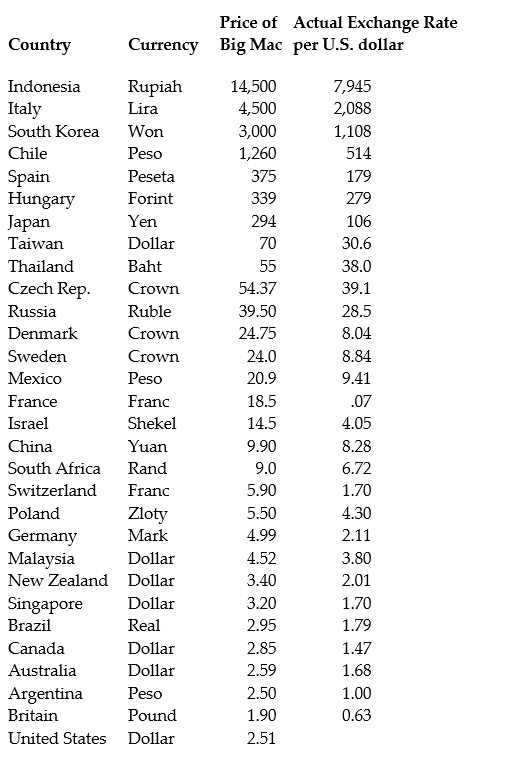The concept of purchasing power parity or PPP ("the idea that similar foreign and domestic goods … should have the same price in terms of the same currency," Abel, A. and B. Bernanke, Macroeconomics, 4^th edition, Boston: Addison Wesley, 476)suggests that the ratio of the Big Mac priced in the local currency to the U.S. dollar price should equal the exchange rate between the two countries. (a)Enter the data into your regression analysis program (EViews, Stata, Excel, SAS, etc.). Calculate the predicted exchange rate per U.S. dollar by dividing the price of a Big Mac in local currency by the U.S. price of a Big Mac ($2.51). (b)Run a regression of the actual exchange rate on the predicted exchange rate. If purchasing power parity held, what would you expect the slope and the intercept of the regression to be? Is the value of the slope and the intercept "far" from the values you would expect to hold under PPP? (c)Plot the actual exchange rate against the predicted exchange rate. Include the 45 degree line in your graph. Which observations might cause the slope and the intercept to differ from zero and one?

Consider the sample regression function Y_i = $\hat { \beta }$ ₀ + $\hat { \beta }$ ₁X_i + $\bar u$ _i. First, take averages on both sides of the equation. Second, subtract the resulting equation from the above equation to write the sample regression function in deviations from means. (For simplicity, you may want to use small letters to indicate deviations from the mean, i.e., z_i = Z_i - $\bar { Z }$ )Finally, illustrate in a two-dimensional diagram with SSR on the vertical axis and the regression slope on the horizontal axis how you could find the least squares estimator for the slope by varying its values through trial and error.

The OLS slope estimator is not defined if there is no variation in the data for the explanatory variable. You are interested in estimating a regression relating earnings to years of schooling. Imagine that you had collected data on earnings for different individuals, but that all these individuals had completed a college education (16 years of education). Sketch what the data would look like and explain intuitively why the OLS coefficient does not exist in this situation.

The regression R² is a measure of

The baseball team nearest to your home town is, once again, not doing well. Given that your knowledge of what it takes to win in baseball is vastly superior to that of management, you want to find out what it takes to win in Major League Baseball (MLB). You therefore collect the winning percentage of all 30 baseball teams in MLB for 1999 and regress the winning percentage on what you consider the primary determinant for wins, which is quality pitching (team earned run average). You find the following information on team performance: Summary of the Distribution of Winning Percentage and Team Earned Run Average for MLB in 1999 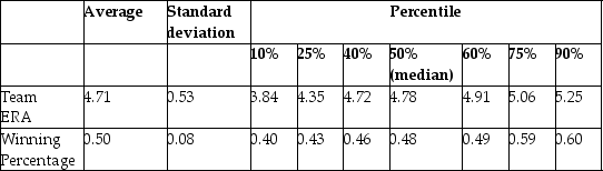(a)What is your expected sign for the regression slope? Will it make sense to interpret the intercept? If not, should you omit it from your regression and force the regression line through the origin? (b)OLS estimation of the relationship between the winning percentage and the team ERA yield the following: $\widehat {\text { Winpct }}$ = 0.9 - 0.10 × teamera , R²=0.49, SER = 0.06, where winpct is measured as wins divided by games played, so for example a team that won half of its games would have Winpct = 0.50. Interpret your regression results. (c)It is typically sufficient to win 90 games to be in the playoffs and/or to win a division. Winning over 100 games a season is exceptional: the Atlanta Braves had the most wins in 1999 with 103. Teams play a total of 162 games a year. Given this information, do you consider the slope coefficient to be large or small? (d)What would be the effect on the slope, the intercept, and the regression R² if you measured Winpct in percentage points, i.e., as (Wins/Games)× 100? (e)Are you impressed with the size of the regression R²? Given that there is 51% of unexplained variation in the winning percentage, what might some of these factors be?

The OLS residuals, $\hat u$ _i, are sample counterparts of the population

Consider the sample regression function $Y _ { i } ^ { * } = \hat { y } _ { 0 } + \hat { y } _ { 1 } X _ { i } ^ { * } + \hat { u _ { i } }$ , where * indicates that the variable has been standardized. What are the units of measurement for the dependent and explanatory variable? Why would you want to transform both variables in this way? Show that the OLS estimator for the intercept equals zero. Next prove that the OLS estimator for the slope in this case is identical to the formula for the least squares estimator where the variables have not been standardized, times the ratio of the sample standard deviation of X and Y, i.e., $\hat { \gamma } _ { 1 } = \hat { \beta } _ { 1 } * \frac { S _ { X } } { S _ { y } }$

The neoclassical growth model predicts that for identical savings rates and population growth rates, countries should converge to the per capita income level. This is referred to as the convergence hypothesis. One way to test for the presence of convergence is to compare the growth rates over time to the initial starting level. (a)If you regressed the average growth rate over a time period (1960-1990)on the initial level of per capita income, what would the sign of the slope have to be to indicate this type of convergence? Explain. Would this result confirm or reject the prediction of the neoclassical growth model? (b)The results of the regression for 104 countries were as follows: $\widehat { g 6090 }$ = 0.019 - 0.0006 × RelProd₆₀ , R² = 0.00007, SER = 0.016, where g6090 is the average annual growth rate of GDP per worker for the 1960-1990 sample period, and RelProd₆₀ is GDP per worker relative to the United States in 1960. Interpret the results. Is there any evidence of unconditional convergence between the countries of the world? Is this result surprising? What other concept could you think about to test for convergence between countries? (c)You decide to restrict yourself to the 24 OECD countries in the sample. This changes your regression output as follows: $\widehat { g 6090 }$ = 0.048 - 0.0404 RelProd₆₀ , R² = 0.82 , SER = 0.0046 How does this result affect your conclusions from above?

E(u_i | X_i)= 0 says that

The standard error of the regression (SER)is defined as follows

The following are all least squares assumptions with the exception of: