Question 1

All of the following are examples of joint hypotheses on multiple regression coefficients, with the exception of

Accepted Answer

A) H0 : ?1 + ?2 = 1 
B) H0 : $\frac { \beta _ { 3 } } { \beta _ { 2 } }$ = ?1 and ?4 = 0 
C) H0 : ?2 = 0 and ?3 = 0 
D) H0 : ?1 = -?2 and ?1 + ?2 = 1 
A) H0 : ?1 + ?2 = 1 
B) H0 : $\frac { \beta _ { 3 } } { \beta _ { 2 } }$ = ?1 and ?4 = 0 
C) H0 : ?2 = 0 and ?3 = 0 
D) H0 : ?1 = -?2 and ?1 + ?2 = 1

Question 2

You have collected data from Major League Baseball (MLB)to find the determinants of winning. You have a general idea that both good pitching and strong hitting are needed to do well. However, you do not know how much each of these contributes separately. To investigate this problem, you collect data for all MLB during 1999 season. Your strategy is to first regress the winning percentage on pitching quality ("Team ERA"), second to regress the same variable on some measure of hitting ("OPS - On-base Plus Slugging percentage"), and third to regress the winning percentage on both.
Summary of the Distribution of Winning Percentage, On Base plus Slugging Percentage,
and Team Earned Run Average for MLB in 1999 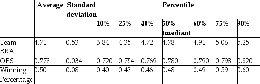  The results are as follows: $\widehat{\text { Winpct} }$ = 0.94 - 0.100 × teamera, R2 = 0.49, SER = 0.06.
(0.08)(0.017) $\widehat{\text { Winpct }}$ = -0.68 + 1.513 × ops, R2=0.45, SER = 0.06.
(0.17)(0.221) $\widehat{\text { Winpct }}$ = -0.19 - 0.099 × teamera + 1.490 × ops, R2=0.92, SER = 0.02.
(0.08)(0.008)(0.126)
(a)Use the t-statistic to test for the statistical significance of the coefficient.
(b)There are 30 teams in MLB. Does the small sample size worry you here when testing for significance?

Accepted Answer

(a)The t-statistics for team ERA and OPS

Question 3

Using the California School data set from your textbook, you decide to run a regression of the average reading score (ScrRead)on the average mathematics score (ScrMaths). The result is as follows, where the numbers in parenthesis are homoskedasticity only standard errors: $\widehat{\text { ScrRead }}$ = 8.47 + 0.9895×ScrMaths
(13.20)(0.0202)
N = 420, R2 = 0.85, SER = 7.8
You believe that the average mathematics score is an unbiased predictor of the average reading score. Consider the above regression to be the unrestricted from which you would calculate SSRUnrestricted . How would you find the SSRRestricted? How many restrictions would have to impose?

Accepted Answer

Since the restricted regression would re

Question 4

Set up the null hypothesis and alternative hypothesis carefully for the following cases:
(a)k = 4, test for all coefficients other than the intercept to be zero
(b)k = 3, test for the slope coefficient of X1 to be unity, and the coefficients on the other explanatory variables to be zero
(c)k = 10, test for the slope coefficient of X1 to be zero, and for the slope coefficients of X2 and X3 to be the same but of opposite sign.
(d)k = 4, test for the slope coefficients to add up to unity

Accepted Answer

(a)H₀ : β₁ = 0, β₂ = 0, β₃= 0, β₄=

Question 5

Let R2unrestricted and R2restricted be 0.4366 and 0.4149 respectively. The difference between the unrestricted and the restricted model is that you have imposed two restrictions. There are 420 observations. The F-statistic in this case is

Accepted Answer

A) 4.61 
B) 8.01 
C) 10.34 
D) 7.71 
A) 4.61 
B) 8.01 
C) 10.34 
D) 7.71

Question 6

The following linear hypothesis can be tested using the F-test with the exception of

Accepted Answer

A) β2 = 1 and β3= β4/β5. 
B) β2 =0. 
C) β1 + β2 = 1 and β3 = -2β4. 
D) β0 = β1 and β1 = 0. 
A) β2 = 1 and β3= β4/β5. 
B) β2 =0. 
C) β1 + β2 = 1 and β3 = -2β4. 
D) β0 = β1 and β1 = 0.

Question 7

To test joint linear hypotheses in the multiple regression model, you need to

Accepted Answer

A) compare the sums of squared residuals from the restricted and unrestricted model. 
B) use the heteroskedasticity-robust F-statistic. 
C) use several t-statistics and perform tests using the standard normal distribution. 
D) compare the adjusted R2 for the model which imposes the restrictions, and the unrestricted model. 
A) compare the sums of squared residuals from the restricted and unrestricted model. 
B) use the heteroskedasticity-robust F-statistic. 
C) use several t-statistics and perform tests using the standard normal distribution. 
D) compare the adjusted R2 for the model which imposes the restrictions, and the unrestricted model.

Question 8

The Solow growth model suggests that countries with identical saving rates and population growth rates should converge to the same per capita income level. This result has been extended to include investment in human capital (education)as well as investment in physical capital. This hypothesis is referred to as the "conditional convergence hypothesis," since the convergence is dependent on countries obtaining the same values in the driving variables. To test the hypothesis, you collect data from the Penn World Tables on the average annual growth rate of GDP per worker (g6090)for the 1960-1990 sample period, and regress it on the (i)initial starting level of GD-P per worker relative to the United States in 1960 (RelProd60), (ii)average population growth rate of the country (n), (iii)average investment share of GDP from 1960 to 1990 (SK - remember investment equals savings), and (iv)educational attainment in years for 1985 (Educ). The results for close to 100 countries is as follows (numbers in parentheses are for heteroskedasticity-robust standard errors): $\widehat { g 6090 }$ = 0.004 - 0.172 × n + 0.133 × SK + 0.002 × Educ - 0.044 × RelProd60,
(0.007)(0.209)(0.015)(0.001)(0.008)
R2=0.537, SER = 0.011
(a)Is the coefficient on this variable significantly different from zero at the 5% level? At the 1% level?
(b)Test for the significance of the other slope coefficients. Should you use a one-sided alternative hypothesis or a two-sided test? Will the decision for one or the other influence the decision about the significance of the parameters? Should you always eliminate variables which carry insignificant coefficients?

Accepted Answer

(a)The coefficient has a t-statistic of

Question 9

To calculate the homoskedasticity-only overall regression F-statistic, you need to compare the SSRrestricted with the SSRunrestricted. Consider the following output from a regression package, which reproduces the regression results of testscores on the student-teacher ratio, the percent of English learners, and the expenditures per student from your textbook:
Dependent Variable: TESTSCR
Method: Least Squares
Date: 07/30/06 Time: 17:55
Sample: 1 420
Included observations: 420 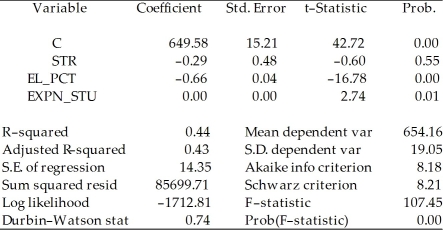  Sum of squared resid corresponds to SSRunrestricted. How are you going to find SSRrestricted?

Accepted Answer

You could simply run a regression of Tes

Question 10

Analyzing a regression using data from a sub-sample of the Current Population Survey with about 4,000 observations, you realize that the regression R2, and the adjusted R2, $\overline { \mathrm { R } }$ 2, are almost identical. Why is that the case? In your textbook, you were told that the regression R2 will almost always increase when you add an explanatory variable, but that the adjusted measure does not have to increase with such an addition. Can this still be true?

Accepted Answer

The difference between the two measures

Question 11

All of the following are correct formulae for the homoskedasticity-only F-statistic, with the exception of

Accepted Answer

A)  $F = \frac { \left( S S R _ { \text {restricted } } - S S R _ { \text {unrestricted } } \right) / q } { S S R _ { \text {unrestricted} } / \left( n - k _ { \text {unrestricted } } - 1 \right) }$ 
B)  $F = \frac { \left( S S R _ { \text {unrestricted } } - S S R _ { \text {restictad } } \right) / q } { S S R _ { \text {restricted} } / \left( n - k _ { \text {restricted } } - 1 \right) }$ 
C)    
D)  $F = \left( \frac { S S R _ { \text {restricted } } } { S S R _ { \text {unrestricted } } } - 1 \right) \times \frac { \left( n - k _ { \text {unrestricted} } - 1 \right) } { q }$ 
A)  $F = \frac { \left( S S R _ { \text {restricted } } - S S R _ { \text {unrestricted } } \right) / q } { S S R _ { \text {unrestricted} } / \left( n - k _ { \text {unrestricted } } - 1 \right) }$ 
B)  $F = \frac { \left( S S R _ { \text {unrestricted } } - S S R _ { \text {restictad } } \right) / q } { S S R _ { \text {restricted} } / \left( n - k _ { \text {restricted } } - 1 \right) }$ 
C)    
D)  $F = \left( \frac { S S R _ { \text {restricted } } } { S S R _ { \text {unrestricted } } } - 1 \right) \times \frac { \left( n - k _ { \text {unrestricted} } - 1 \right) } { q }$

Question 12

Explain carefully why testing joint hypotheses simultaneously, using the F-statistic, does not necessarily yield the same conclusion as testing them sequentially ("one at a time" method), using a series of t-statistics.

Accepted Answer

Testing a joint hypothesis sequentially

Question 13

You have estimated the relationship between testscores and the student-teacher ratio under the assumption of homoskedasticity of the error terms. The regression output is as follows: $\widehat{\text { TestScore} }$ = 698.9 - 2.28 × STR, and the standard error on the slope is 0.48. The homoskedasticity-only "overall" regression F- statistic for the hypothesis that the Regression R2 is zero is approximately

Accepted Answer

A) 0.96 
B) 1.96 
C) 22.56 
D) 4.75 
A) 0.96 
B) 1.96 
C) 22.56 
D) 4.75

Question 14

The confidence interval for a single coefficient in a multiple regression

Accepted Answer

A) makes little sense because the population parameter is unknown. 
B) should not be computed because there are other coefficients present in the model. 
C) contains information from a large number of hypothesis tests. 
D) should only be calculated if the regression R2 is identical to the adjusted R2. 
A) makes little sense because the population parameter is unknown. 
B) should not be computed because there are other coefficients present in the model. 
C) contains information from a large number of hypothesis tests. 
D) should only be calculated if the regression R2 is identical to the adjusted R2.

Question 15

Looking at formula (7.13)in your textbook for the homoskedasticity-only F-statistic, 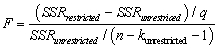  give three conditions under which, ceteris paribus, you would find a large value, and hence would be likely to reject the null hypothesis.

Accepted Answer

The F-statistic will be larger for (i)la

Question 16

Consider the following two models to explain testscores.
Model 1:
Dependent Variable: TESTSCR
Method: Least Squares
Date: 07/31/06 Time: 17:52
Sample: 1 420
Included observations: 420   Model 2:
Dependent Variable: TESTSCR
Method: Least Squares
Date: 07/31/06 Time: 17:56
Sample: 1 420
Included observations: 420 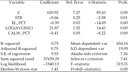  Explain why you cannot use the F-test in this situation to discriminate between Model 1 and Model 2.

Accepted Answer

Neither model is contained ("nested")in

Question 17

The critical value of F4,∞ at the 5% significance level is

Accepted Answer

A) 3.84 
B) 2.37 
C) 1.94 
D) Cannot be calculated because in practice you will not have infinite number of observations 
A) 3.84 
B) 2.37 
C) 1.94 
D) Cannot be calculated because in practice you will not have infinite number of observations

Question 18

If you wanted to test, using a 5% significance level, whether or not a specific slope coefficient is equal to one, then you should

Accepted Answer

A) subtract 1 from the estimated coefficient, divide the difference by the standard error, and check if the resulting ratio is larger than 1.96. 
B) add and subtract 1.96 from the slope and check if that interval includes 1. 
C) see if the slope coefficient is between 0.95 and 1.05. 
D) check if the adjusted R2 is close to 1. 
A) subtract 1 from the estimated coefficient, divide the difference by the standard error, and check if the resulting ratio is larger than 1.96. 
B) add and subtract 1.96 from the slope and check if that interval includes 1. 
C) see if the slope coefficient is between 0.95 and 1.05. 
D) check if the adjusted R2 is close to 1.

Question 19

Consider the following regression using the California School data set from your textbook. $\widehat{\text { TestScore }}$ = 681.44 - 0.61LchPct
n=420, R2=0.75, SER=9.45
where TestScore is the test score and LchPct is the percent of students eligible for subsidized lunch (average = 44.7, max = 100, min = 0).
a. What is the effect of a 20 percentage point increase in the student eligible for subsidized lunch?
b. Your textbook started with the following regression in Chapter 4: $\widehat{\text { TestScore} }$ = 698.9 - 2.28STR
n=420, R2=0.051, SER=18.58
where STR is the student teacher ratio.
Your textbook tells you that in the multiple regression framework considered, the percentage of students eligible for subsidized lunch is a control variable, while the student teacher ratio is the variable of interest. Given that the regression R2 is so much higher for the first equation than for the second equation, shouldn't the role of the two variables be reversed? That is, shouldn't the student teacher ratio be the control variable while the percent of students eligible for subsidized lunch be the variable of interest?

Accepted Answer

a. The effect would be a 12.2 test score

Question 20

The administration of your university/college is thinking about implementing a policy of coed floors only in dormitories. Currently there are only single gender floors. One reason behind such a policy might be to generate an atmosphere of better "understanding" between the sexes. The Dean of Students (DoS)has decided to investigate if such a behavior results in more "togetherness" by attempting to find the determinants of the gender composition at the dinner table in your main dining hall, and in that of a neighboring university, which only allows for coed floors in their dorms. The survey includes 176 students, 63 from your university/college, and 113 from a neighboring institution.
The Dean's first problem is how to define gender composition. To begin with, the survey excludes single persons' tables, since the study is to focus on group behavior. The Dean also eliminates sports teams from the analysis, since a large number of single-gender students will sit at the same table. Finally, the Dean decides to only analyze tables with three or more students, since she worries about "couples" distorting the results. The Dean finally settles for the following specification of the dependent variable:
GenderComp = $\mid ( 50 \% - \% \text { of Male Students at Table } ) \mid$ Where " $| Z |$ " stands for absolute value of Z. The variable can take on values from zero to fifty.
After considering various explanatory variables, the Dean settles for an initial list of eight, and estimates the following relationship, using heteroskedasticity-robust standard errors (this Dean obviously has taken an econometrics course earlier in her career and/or has an able research assistant): $\text { h }$ = 30.90 - 3.78 × Size - 8.81 × DCoed + 2.28 × DFemme +2.06 × DRoommate
(7.73)(0.63)(2.66)(2.42)(2.39)
- 0.17 × DAthlete + 1.49 × DCons - 0.81 SAT + 1.74 × SibOther, R2=0.24, SER = 15.50
(3.23)(1.10)(1.20)(1.43)
where Size is the number of persons at the table minus 3; DCoed is a binary variable, which takes on the value of 1 if you live on a coed floor; DFemme is a binary variable, which is 1 for females and zero otherwise; DRoommate is a binary variable which equals 1 if the person at the table has a roommate and is zero otherwise; DAthlete is a binary variable which is 1 if the person at the table is a member of an athletic varsity team; DCons is a variable which measures the political tendency of the person at the table on a seven-point scale, ranging from 1 being "liberal" to 7 being "conservative"; SAT is the SAT score of the person at the table measured on a seven-point scale, ranging from 1 for the category "900-1000" to 7 for the category "1510 and above"; and increasing by one for 100 point increases; and SibOther is the number of siblings from the opposite gender in the family the person at the table grew up with.
(a)Indicate which of the coefficients are statistically significant.
(b)Based on the above results, the Dean decides to specify a more parsimonious form by eliminating the least significant variables. Using the F-statistic for the null hypothesis that there is no relationship between the gender composition at the table and DFemme, DRoommate, DAthlete, and SAT, the regression package returns a value of 1.10. What are the degrees of freedom for the statistic? Look up the 1% and 5% critical values from the F- table and make a decision about the exclusion of these variables based on the critical values.
(c)The Dean decides to estimate the following specification next:   = 29.07 - 3.80 × Size - 9.75 × DCoed + 1.50 × DCons + 1.97 × SibOther,
(3.75)(0.62)(1.04)(1.04)(1.44)
R2=0.22 SER = 15.44
Calculate the t-statistics for the coefficients and discuss whether or not the Dean should attempt to simplify the specification further. Based on the results, what might some of the comments be that she will write up for the other senior administrators of your college? What are some of the potential flaws in her analysis? What other variables do you think she should have considered as explanatory factors?

Accepted Answer

(a)Only the constant, Size, and DCoed ar

All of the following are examples of joint hypotheses on multiple regression coefficients, with the exception of

Let R²_unrestricted and R²_restricted be 0.4366 and 0.4149 respectively. The difference between the unrestricted and the restricted model is that you have imposed two restrictions. There are 420 observations. The F-statistic in this case is

The following linear hypothesis can be tested using the F-test with the exception of

To test joint linear hypotheses in the multiple regression model, you need to

All of the following are correct formulae for the homoskedasticity-only F-statistic, with the exception of

Explain carefully why testing joint hypotheses simultaneously, using the F-statistic, does not necessarily yield the same conclusion as testing them sequentially ("one at a time" method), using a series of t-statistics.

The confidence interval for a single coefficient in a multiple regression

Looking at formula (7.13)in your textbook for the homoskedasticity-only F-statistic, give three conditions under which, ceteris paribus, you would find a large value, and hence would be likely to reject the null hypothesis.

The critical value of F_4,_∞ at the 5% significance level is

If you wanted to test, using a 5% significance level, whether or not a specific slope coefficient is equal to one, then you should

Economic Questions and Data

Review of Probability

Review of Statistics

Linear Regression With One Regressor

Regression With a Single Regressor: Hypothesis Tests and Confidence Intervals

Linear Regression With Multiple Regressors

Nonlinear Regression Functions

Assessing Studies Based on Multiple Regression

Regression With Panel Data

Regression With a Binary Dependent Variable

Instrumental Variables Regression

Experiments and Quasi-Experiments

Introduction to Time Series Regression and Forecasting

Estimation of Dynamic Causal Effects

Additional Topics in Time Series Regression

The Theory of Linear Regression With One Regressor

The Theory of Multiple Regression

Filters

Exam 7: Hypothesis Tests and Confidence Intervals in Multiple Regression

All of the following are examples of joint hypotheses on multiple regression coefficients, with the exception of

Let R2unrestricted and R2restricted be 0.4366 and 0.4149 respectively. The difference between the unrestricted and the restricted model is that you have imposed two restrictions. There are 420 observations. The F-statistic in this case is

The following linear hypothesis can be tested using the F-test with the exception of

To test joint linear hypotheses in the multiple regression model, you need to

All of the following are correct formulae for the homoskedasticity-only F-statistic, with the exception of

Explain carefully why testing joint hypotheses simultaneously, using the F-statistic, does not necessarily yield the same conclusion as testing them sequentially ("one at a time" method), using a series of t-statistics.

The confidence interval for a single coefficient in a multiple regression

Looking at formula (7.13)in your textbook for the homoskedasticity-only F-statistic, give three conditions under which, ceteris paribus, you would find a large value, and hence would be likely to reject the null hypothesis.

The critical value of F4,∞ at the 5% significance level is

If you wanted to test, using a 5% significance level, whether or not a specific slope coefficient is equal to one, then you should

Economic Questions and Data

Review of Probability

Review of Statistics

Linear Regression With One Regressor

Regression With a Single Regressor: Hypothesis Tests and Confidence Intervals

Linear Regression With Multiple Regressors

Nonlinear Regression Functions

Assessing Studies Based on Multiple Regression

Regression With Panel Data

Regression With a Binary Dependent Variable

Instrumental Variables Regression

Experiments and Quasi-Experiments

Introduction to Time Series Regression and Forecasting

Estimation of Dynamic Causal Effects

Additional Topics in Time Series Regression

The Theory of Linear Regression With One Regressor

The Theory of Multiple Regression

Filters

Let R²_unrestricted and R²_restricted be 0.4366 and 0.4149 respectively. The difference between the unrestricted and the restricted model is that you have imposed two restrictions. There are 420 observations. The F-statistic in this case is

The critical value of F_4,_∞ at the 5% significance level is