Exam 7: Hypothesis Tests and Confidence Intervals in Multiple Regression
Exam 1: Economic Questions and Data17 Questions
Exam 2: Review of Probability70 Questions
Exam 3: Review of Statistics65 Questions
Exam 4: Linear Regression With One Regressor65 Questions
Exam 5: Regression With a Single Regressor: Hypothesis Tests and Confidence Intervals59 Questions
Exam 6: Linear Regression With Multiple Regressors65 Questions
Exam 7: Hypothesis Tests and Confidence Intervals in Multiple Regression64 Questions
Exam 8: Nonlinear Regression Functions63 Questions
Exam 9: Assessing Studies Based on Multiple Regression65 Questions
Exam 10: Regression With Panel Data50 Questions
Exam 11: Regression With a Binary Dependent Variable50 Questions
Exam 12: Instrumental Variables Regression50 Questions
Exam 13: Experiments and Quasi-Experiments50 Questions
Exam 14: Introduction to Time Series Regression and Forecasting50 Questions
Exam 15: Estimation of Dynamic Causal Effects50 Questions
Exam 16: Additional Topics in Time Series Regression50 Questions
Exam 17: The Theory of Linear Regression With One Regressor49 Questions
Exam 18: The Theory of Multiple Regression50 Questions
Select questions type
You are presented with the following output from a regression package, which reproduces the regression results of testscores on the student-teacher ratio from your textbook
Dependent Variable: TESTSCR
Method: Least Squares
Date: 07/30/06 Time: 17:44
Sample: 1 420
Included observations: 420 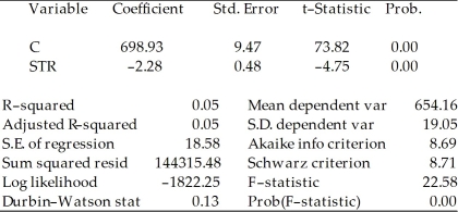 Std. Error are homoskedasticity only standard errors.
a)What is the relationship between the t-statistic on the student-teacher ratio coefficient and the F-statistic?
b)Next, two explanatory variables, the percent of English learners (EL_PCT)and expenditures per student (EXPN_STU)are added. The output is listed as below. What is the relationship between the three t-statistics for the slopes and the homoskedasticity-only F-statistic now?
Dependent Variable: TESTSCR
Method: Least Squares
Date: 07/30/06 Time: 17:55
Sample: 1 420
Included observations: 420
Std. Error are homoskedasticity only standard errors.
a)What is the relationship between the t-statistic on the student-teacher ratio coefficient and the F-statistic?
b)Next, two explanatory variables, the percent of English learners (EL_PCT)and expenditures per student (EXPN_STU)are added. The output is listed as below. What is the relationship between the three t-statistics for the slopes and the homoskedasticity-only F-statistic now?
Dependent Variable: TESTSCR
Method: Least Squares
Date: 07/30/06 Time: 17:55
Sample: 1 420
Included observations: 420 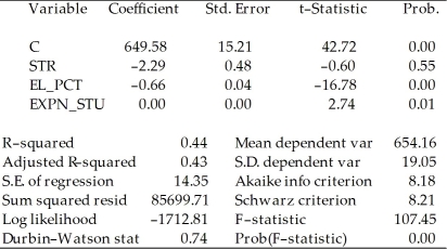
(Essay)
4.8/5  (32)
(32)
Your textbook has emphasized that testing two hypothesis sequentially is not the same as testing them simultaneously. Consider the following confidence set below, where you are testing the hypothesis that H0 : β5 = 0, β6 = 0. 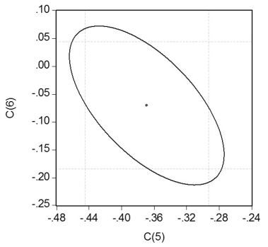 Your statistical package has also generated a dotted area, which corresponds to drawing two confidence intervals for the respective coefficients. For each case where the ellipse does not coincide in area with the corresponding rectangle, indicate what your decision would be if you relied on the two confidence intervals vs. the ellipse generated by the F-statistic.
(Essay)
4.9/5 (32)
At a mathematical level, if the two conditions for omitted variable bias are satisfied, then
(Multiple Choice)
4.8/5 (33)
Adding the Percent of English Speakers (PctEL)to the Student Teacher Ratio (STR)in your textbook reduced the coefficient for STR from 2.28 to 1.10 with a standard error of 0.43. Construct a 90% and 99% confidence interval to test the hypothesis that the coefficient of STR is 2.28.
(Essay)
4.9/5 (33)
If the estimates of the coefficients of interest change substantially across specifications,
(Multiple Choice)
4.8/5 (34)
You have collected data for 104 countries to address the difficult questions of the determinants for differences in the standard of living among the countries of the world. You recall from your macroeconomics lectures that the neoclassical growth model suggests that output per worker (per capita income)levels are determined by, among others, the saving rate and population growth rate. To test the predictions of this growth model, you run the following regression: = 0.339 - 12.894 × n + 1.397 × SK, R2=0.621, SER = 0.177
(0.068)(3.177)(0.229)
where RelPersInc is GDP per worker relative to the United States, n is the average population growth rate, 1980-1990, and SK is the average investment share of GDP from 1960 to 1990 (remember investment equals saving). Numbers in parentheses are for heteroskedasticity-robust standard errors.
(a)Calculate the t-statistics and test whether or not each of the population parameters are significantly different from zero.
(b)The overall F-statistic for the regression is 79.11. What is the critical value at the 5% and 1% level? What is your decision on the null hypothesis?
(c)You remember that human capital in addition to physical capital also plays a role in determining the standard of living of a country. You therefore collect additional data on the average educational attainment in years for 1985, and add this variable (Educ)to the above regression. This results in the modified regression output: = 0.046 - 5.869 × n + 0.738 × SK + 0.055 × Educ, R2=0.775, SER = 0.1377
(0.079)(2.238)(0.294)(0.010)
How has the inclusion of Educ affected your previous results?
(d)Upon checking the regression output, you realize that there are only 86 observations, since data for Educ is not available for all 104 countries in your sample. Do you have to modify some of your statements in (d)?
(Essay)
4.8/5 (37)
Trying to remember the formula for the homoskedasticity-only F-statistic, you forgot whether you subtract the restricted SSR from the unrestricted SSR or the other way around. Your professor has provided you with a table containing critical values for the F distribution. How can this be of help?
(Essay)
4.9/5 (32)
The homoskedasticity-only F-statistic and the heteroskedasticity-robust F-statistic typically are
(Multiple Choice)
4.8/5 (42)
Consider the following multiple regression model
Yi = ?0 + ?1X1i + ?2X2i + ?3X3i + ui
You want to consider certain hypotheses involving more than one parameter, and you know that the regression error is homoskedastic. You decide to test the joint hypotheses using the homoskedasticity-only F-statistics. For each of the cases below specify a restricted model and indicate how you would compute the F-statistic to test for the validity of the restrictions.
(a)?1 = -?2; ?3 = 0
(b)?1 + ?2 + ?3 = 1
(c)?1 = ?2; ?3 = 0
(Essay)
4.8/5 (36)
Consider a regression with two variables, in which X1i is the variable of interest and X2i is the control variable. Conditional mean independence requires
(Multiple Choice)
4.9/5 (37)
A subsample from the Current Population Survey is taken, on weekly earnings of individuals, their age, and their gender. You have read in the news that women make 70 cents to the $1 that men earn. To test this hypothesis, you first regress earnings on a constant and a binary variable, which takes on a value of 1 for females and is 0 otherwise. The results were: = 570.70 - 170.72 × Female, R2=0.084, SER = 282.12.
(9.44)(13.52)
(a)Perform a difference in means test and indicate whether or not the difference in the mean salaries is significantly different. Justify your choice of a one-sided or two-sided alternative test. Are these results evidence enough to argue that there is discrimination against females? Why or why not? Is it likely that the errors are normally distributed in this case? If not, does that present a problem to your test?
(b)Test for the significance of the age and gender coefficients. Why do you think that age plays a role in earnings determination?
(Essay)
4.9/5 (29)
The OLS estimators of the coefficients in multiple regression will have omitted variable bias
(Multiple Choice)
4.9/5 (32)
Using the 420 observations of the California School data set from your textbook, you estimate the following relationship: = 681.44 - 0.61LchPct
n=420, R2=0.75, SER=9.45
where TestScore is the test score and LchPct is the percent of students eligible for subsidized lunch (average = 44.7, max = 100, min = 0).
a. Interpret the regression result.
b. In your interpretation of the slope coefficient in (a)above, does it matter if you start your explanation with "for every x percent increase" rather than "for every x percentage point increase"?
c. The "overall" regression F-statistic is 1149.57. What are the degrees of freedom for this statistic?
d. Find the critical value of the F-statistic at the 1% significance level. Test the null hypothesis that the regression R2= 0.
e. The above equation was estimated using heteroskedasticity robust standard errors. What is the standard error for the slope coefficient?
(Essay)
4.8/5 (29)
Consider the following regression output where the dependent variable is testscores and the two explanatory variables are the student-teacher ratio and the percent of English learners: = 698.9 - 1.10×STR - 0.650×PctEL. You are told that the t-statistic on the student-teacher ratio coefficient is 2.56. The standard error therefore is approximately
(Multiple Choice)
4.9/5 (32)
The formula for the standard error of the regression coefficient, when moving from one explanatory variable to two explanatory variables,
(Multiple Choice)
4.7/5 (41)
Females, on average, are shorter and weigh less than males. One of your friends, who is a pre-med student, tells you that in addition, females will weigh less for a given height. To test this hypothesis, you collect height and weight of 29 female and 81 male students at your university. A regression of the weight on a constant, height, and a binary variable, which takes a value of one for females and is zero otherwise, yields the following result: = -229.21 - 6.36 × Female + 5.58 × Height, R2=0.50, SER = 20.99 (43.39)(5.74)(0.62)
where Studentw is weight measured in pounds and Height is measured in inches (heteroskedasticity-robust standard errors in parentheses).
Calculate t-statistics and carry out the hypothesis test that females weigh the same as males, on average, for a given height, using a 10% significance level. What is the alternative hypothesis? What is the p-value? What critical value did you use?
(Essay)
4.9/5 (34)
In the process of collecting weight and height data from 29 female and 81 male students at your university, you also asked the students for the number of siblings they have. Although it was not quite clear to you initially what you would use that variable for, you construct a new theory that suggests that children who have more siblings come from poorer families and will have to share the food on the table. Although a friend tells you that this theory does not pass the "straight-face" test, you decide to hypothesize that peers with many siblings will weigh less, on average, for a given height. In addition, you believe that the muscle/fat tissue composition of male bodies suggests that females will weigh less, on average, for a given height. To test these theories, you perform the following regression: = -229.92 - 6.52 × Female + 0.51 × Sibs+ 5.58 × Height,
(44.01)(5.52)(2.25)(0.62)
R2=0.50, SER = 21.08
where Studentw is in pounds, Height is in inches, Female takes a value of 1 for females and is 0 otherwise, Sibs is the number of siblings (heteroskedasticity-robust standard errors in parentheses).
(a)Carrying out hypotheses tests using the relevant t-statistics to test your two claims separately, is there strong evidence in favor of your hypotheses? Is it appropriate to use two separate tests in this situation?
(b)You also perform an F-test on the joint hypothesis that the two coefficients for females and siblings are zero. The calculated F-statistic is 0.84. Find the critical value from the F-table. Can you reject the null hypothesis? Is it possible that one of the two parameters is zero in the population, but not the other?
(c)You are now a bit worried that the entire regression does not make sense and therefore also test for the height coefficient to be zero. The resulting F-statistic is 57.25. Does that prove that there is a relationship between weight and height?
(Essay)
4.7/5 (43)
When there are two coefficients, the resulting confidence sets are
(Multiple Choice)
4.8/5 (32)
Filters
- Essay(0)
- Multiple Choice(0)
- Short Answer(0)
- True False(0)
- Matching(0)