Question 1

A vector autoregression

Accepted Answer

A) is the ADL model with an AR process in the error term. 
B) is the same as a univariate autoregression. 
C) is a set of k time series regressions, in which the regressors are lagged values of all k series. 
D) involves errors that are autocorrelated but can be written in vector format. 
A) is the ADL model with an AR process in the error term. 
B) is the same as a univariate autoregression. 
C) is a set of k time series regressions, in which the regressors are lagged values of all k series. 
D) involves errors that are autocorrelated but can be written in vector format.

Question 2

You have collected quarterly Canadian data on the unemployment and the inflation rate from 1962:I to 2001:IV. You want to re-estimate the ADL(3,1)formulation of the Phillips curve using a GARCH(1,1)specification. The results are as follows: $\widehat{\Delta I n f}_{t}=1.17-.56 \Delta I n f_{t-1}-.47 \Delta I n f_{t-2}-.31 \Delta I n f_{t-3}-.13 \text { Unempt-1 }$
(.48) (.08)$\quad$(.10)$\quad$(.09)$\quad$$ (.06) $
$\hat{\sigma}_{t}^{2}=.86+.27 u_{t-1}^{2}+.53 \sigma_{t-1}^{2} .$
$(.40)(.11)$$\quad$(.15)
(a)Test the two coefficients for $u _ { t - 1 } ^ { 2 }$ and $\sigma _ { t - 1 } ^ { 2 }$ in the GARCH model individually for statistical significance.
(b)Estimating the same equation by OLS results in $\widehat{\Delta I n f}_{t}=1.19-.51 \Delta I n f_{t-1}-.47 \Delta I n f_{t-2}-.28 \Delta I n f_{t-3}-.16 U_{n e m p t-1}$
(.54) (.10)$\quad$(.11)$\quad$(.08)$\quad$$ (.07) $
Briefly compare the estimates. Which of the two methods do you prefer?
(c)Given your results from the test in (a), what can you say about the variance of the error terms in the Phillips Curve for Canada?
(d)The following figure plots the residuals along with bands of plus or minus one predicted standard deviation (that is, ± $\widehat{\sigma _ { t }}$ )based on the GARCH(1,1)model. 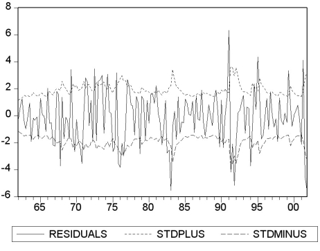  Describe what you see.

Accepted Answer

(a)The two t-statistics are 2.46 and 3.5

Question 3

The dynamic OLS (DOLS)estimator of the cointegrating coefficient, if Yt and Xt are cointegrated,

Accepted Answer

A) is efficient in large samples 
B) statistical inference about the cointegrating coefficient is valid 
C) the t-statistic constructed using the DOLS estimator with HAC standard errors has a standard normal distribution in large samples 
D) all of the above 
A) is efficient in large samples 
B) statistical inference about the cointegrating coefficient is valid 
C) the t-statistic constructed using the DOLS estimator with HAC standard errors has a standard normal distribution in large samples 
D) all of the above

Question 4

Your textbook states that there "are three ways to decide if two variables can plausibly be modeled as cointegrated: use expert knowledge and economic theory, graph the series and see whether they appear to have a common stochastic trend, and perform statistical tests for cointegration. All three ways should be used in practice." Accordingly you set out to check whether (the log of)consumption and (the log of)personal disposable income are cointegrated. You collect data for the sample period 1962:I to 1995:IV and plot the two variables. 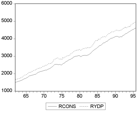  (a)Using the first two methods to examine the series for cointegration, what do you think the likely answer is?
(b)You begin your numerical analysis by testing for a stochastic trend in the variables, using an Augmented Dickey-Fuller test. The t-statistic for the coefficient of interest is as follows: $\begin{array}{|c|c|c|c|c|}\hline \text { Variable with } & \operatorname{Ln} Y p d & \Delta \operatorname{Ln} Y p d & \operatorname{LnC} & \Delta \operatorname{LnC} \
\text { lag of } 1 & & & & \
\hline \text { t-statistic } & -1.93 & -5.24 & -2.20 & -4.31\\hline
\end{array}$ where LnYpd is (the log of)personal disposable income, and LnC is (the log of)real consumption. The estimated equation included an intercept for the two growth rates, and, in addition, a deterministic trend for the level variables. For each case make a decision about the stationarity of the variables based on the critical value of the Augmented Dickey-Fuller test statistic. Why do you think a trend was included for level variables?
(c)Using the first step of the EG-ADF procedure, you get the following result: $\widehat{\ln \mathrm { C }}$ t = -0.24 + 1.017 lnYpdt
Should you interpret this equation? Would you be impressed if you were told that the regression R2 was 0.998 and that the t-statistic for the slope was 266.06? Why or why not?
(d)The Dickey-Fuller test for the residuals for the cointegrating regressions results in a t-statistic of
(-3.64). State the null and alternative hypothesis and make a decision based on the result.
(e)You want to investigate if the slope of the cointegrating vector is one. To do so, you use the DOLS estimator and HAC standard errors. The slope coefficient is 1.024 with a standard error of 0.009. Can you reject the null hypothesis that the slope equals one?

Accepted Answer

(a)There are economic theories which pos

Question 5

Consider the GARCH(1,1)model $\sigma _ { t } ^ { 2 }$ = ?0 + ?1
  $u _ { t - 1 } ^ { 2 }$ + ?1
  $\sigma _ { t - 1 } ^ { 2 }$ Show that this model can be rewritten as $\sigma _ { t } ^ { 2 }$ = $\frac { \alpha _ { 0 } } { 1 - \phi _ { 1 } }$ + ?1( $u _ { t - 1 } ^ { 2 }$ + ?1
  $u _ { t - 2 } ^ { 2 }$ + $\phi _ { 1 } ^ { 2 }$ $u _ { t - 3 } ^ { 2 }$ + $\phi _ { 1 } ^ { 3 }$ $u _ { t - 4 } ^ { 2 }$ + ...). (Hint: use the GARCH(1,1)model but specify it for $\phi _ { t - 1 } ^ { 2 }$ ; substitute this expression into the original specification, and so on.)Explain intuitively the meaning of the resulting formulation.

Accepted Answer

\[\begin{aligned}
\sigma _ { t } ^ { 2

Question 6

What role does the concept of cointegration and the order of integration play in modeling the relationship between variables? Explain how tests of cointegration work.

Accepted Answer

Cointegration between two or more variab

Question 7

The DOLS estimator has the following property if Xt and Yt are cointegrated:

Accepted Answer

A) it is BLUE even in small samples. 
B) it is efficient in large samples. 
C) it has a standard normal distribution when homoskedasticity-only standard errors are used. 
D) it has a non-normal distribution in large samples when HAC standard errors are used. 
A) it is BLUE even in small samples. 
B) it is efficient in large samples. 
C) it has a standard normal distribution when homoskedasticity-only standard errors are used. 
D) it has a non-normal distribution in large samples when HAC standard errors are used.

Question 8

The order of integration

Accepted Answer

A) can never be zero. 
B) is the number of times that the series needs to be differenced for it to be stationary. 
C) is the value of φ1 in the quasi difference(ΔYt - φ1Yt-1). 
D) depends on the number of lags in the VAR specification. 
A) can never be zero. 
B) is the number of times that the series needs to be differenced for it to be stationary. 
C) is the value of φ1 in the quasi difference(ΔYt - φ1Yt-1). 
D) depends on the number of lags in the VAR specification.

Question 9

The EG-ADF test

Accepted Answer

A) is the similar to the DF-GLS test 
B) is a test for cointegration 
C) has as a limitation that it can only test if two variables, but not more than two, are cointegrated 
D) uses the ADF in the second step of its procedure 
A) is the similar to the DF-GLS test 
B) is a test for cointegration 
C) has as a limitation that it can only test if two variables, but not more than two, are cointegrated 
D) uses the ADF in the second step of its procedure

Question 10

One advantage of forecasts based on a VAR rather than separately forecasting the variables involved is

Accepted Answer

A) that VAR forecasts are easier to calculate. 
B) you typically have knowledge of future values of at least one of the variables involved. 
C) it can help to make the forecasts mutually consistent. 
D) that VAR involves panel data. 
A) that VAR forecasts are easier to calculate. 
B) you typically have knowledge of future values of at least one of the variables involved. 
C) it can help to make the forecasts mutually consistent. 
D) that VAR involves panel data.

Question 11

For the United States, there is somewhat conflicting evidence whether or not the inflation rate has a unit autoregressive root. For example, for the sample period 1962:I to 1999:IV using the ADF statistic, you cannot reject at the 5% significance level that inflation contains a stochastic trend. However the null hypothesis can be rejected at the 10% significance level. The DF-GLS test rejects the null hypothesis at the five percent level. This result turns out to be sensitive to the number of lags chosen and the sample period.
(a)Somewhat intrigued by these findings, you decide to repeat the exercise using Canadian data. Letting the AIC choose the lag length of the ADF regression, which turns out to be three, the ADF statistic is
(-1.91). What is your decision regarding the null hypothesis?
(b)You also calculate the DF-GLS statistic, which turns out to be (-1.23). Can you reject the null hypothesis in this case?
(c)Is it possible for the two test statistics to yield different answers and if so, why?

Accepted Answer

(a)For the Canadian data, the null hypot

Question 12

Unit root tests

Accepted Answer

A) use the standard normal distribution since they are based on the t-statistic. 
B) cannot use the standard normal distribution for statistical inference. As a result the ADF statistic has its own special table of critical values. 
C) can use the standard normal distribution only when testing that the level variable is stationary, but not the difference variable. 
D) can use the standard normal distribution but only if HAC standard errors were computed. 
A) use the standard normal distribution since they are based on the t-statistic. 
B) cannot use the standard normal distribution for statistical inference. As a result the ADF statistic has its own special table of critical values. 
C) can use the standard normal distribution only when testing that the level variable is stationary, but not the difference variable. 
D) can use the standard normal distribution but only if HAC standard errors were computed.

Question 13

The lag length in a VAR using the BIC proceeds as follows: Among a set of candidate values of p, the estimated lag length xxxis the value of p

Accepted Answer

A) For which the BIC exceeds the AIC 
B) That maximizes BIC(p) 
C) Cannot be determined here since a VAR is a system of equations, not a single one 
D) That minimizes BIC(p) 
A) For which the BIC exceeds the AIC 
B) That maximizes BIC(p) 
C) Cannot be determined here since a VAR is a system of equations, not a single one 
D) That minimizes BIC(p)

Question 14

You have collected quarterly data for the unemployment rate (Unemp)in the United States, using a sample period from 1962:I (first quarter)to 2009:IV (the data is collected at a monthly frequency, but you have taken quarterly averages).
a. Does economic theory suggest that the unemployment rate should be stationary?
b. Testing the unemployment rate for stationarity, you run the following regression (where the lag length was determined using the BIC; using the AIC instead does not change the outcome of the test, even though it chooses 9 lags of the LHS variable): 
$\begin{array} { c } 
\widehat { \text { Unemp } _ { \mathrm { t } } } = 0.217 - 0.035 \text { Unemp } _ { \mathrm { t } - 1 } + 0.689 \Delta \text { Unemp } _ { \mathrm { t } - 1 } \
\left( \begin{array} { l l l } 
( 0.01 ) & 0.0012&(0.054
\end{array} \right)
\end{array}$
Use the ADF statistic with an intercept only to test for stationarity. What is your decision?
c.The standard errors reported above were homoskedasticity-only standard errors. Do you think you could potentially improve on inference by allowing for HAC standard errors?
d. An alternative test for a unit root, the DF-GLS, produces a test statistic of -2.75. Find the critical value and decide whether or not to reject the null hypothesis. If the decision is different from (c), is there any reason why you might prefer the DF-GLS test over the ADF test?

Accepted Answer

a. In macroeconomics or labor economics,

Question 15

?2Yt

Accepted Answer

A) = ?Yt - ?Yt-1. 
B) = $Y _ { t } ^ { 2 }$ - $Y _ { t - 1 } ^ { 2 }$ 
C) = ?Yt -?Yt-2. 
D) = Yt - Yt-2. 
A) = ?Yt - ?Yt-1. 
B) = $Y _ { t } ^ { 2 }$ - $Y _ { t - 1 } ^ { 2 }$ 
C) = ?Yt -?Yt-2. 
D) = Yt - Yt-2.

Question 16

Purchasing power parity (PPP), postulates that the exchange rate between two countries equals the ratio of the respective price indexes or ExchRate = $\frac { P f } { P }$ (where ExchRate is the foreign exchange rate between the two countries, and P represents the price index, with f indicating the foreign country). The long-run version of PPP implies that that the exchange rate and the price ratio share a common trend.
(a)You collect monthly foreign exchange rate data from 1974:1 to 2002:4 for the U.S./U.K. exchange rate ($/£)and you collect data on the Consumer Price Index for both countries. Explain how you would used the Engle-Granger test statistic to investigate the long-run PPP hypothesis.
(b)One of your peers explains that there may be an easier way to test for the validity of PPP. She suggests to simply test whether or not the "real" exchange rate, or competitiveness, is stationary. (The real exchange rate is given by ExchRate × $\frac { P f } { P }$ )Is she correct? Explain. How would you implement her suggestion? Which alternative test-statistic is available?

Accepted Answer

(a)Using the Engle-Granger two step proc

Question 17

There has been much talk recently about the convergence of inflation rates between many of the OECD economies. You want to see if there is evidence of this closer to home by checking whether or not Canada's inflation rate and the United States' inflation rate are cointegrated.
(a)You begin your numerical analysis by testing for a stochastic trend in the variables, using an Augmented Dickey-Fuller test. The t-statistic for the coefficient of interest is as follows: $\begin{array}{|c|c|c|c|c|}\hline \text { Variable with } & \text { InfCan } & \Delta \operatorname{InfCan} & \text { InfUS } & \Delta \operatorname{Inf} U \mathrm{~S} \
\text { lag of } 1 & & & & \
\hline \text { t-statistic } & -1.93 & -5.24 & -2.20 & -4.31\\hline
\end{array}$ where InfCan is the Canadian inflation rate, and InfUS is the United States inflation rate. The estimated equation included an intercept. For each case make a decision about the stationarity of the variables based on the critical value of the Augmented Dickey-Fuller test statistic.
(b)Your test for cointegration results in a EG-ADF statistic of (-7.34). Can you reject the null hypothesis of a unit root for the residuals from the cointegrating regression?
(c)Using a working hypothesis that the two inflation rates are cointegrated, you want to test whether or not the slope coefficient equals one. To do so you estimate the cointegrating equation using the DOLS estimator with HAC standard errors. The coefficient on the U.S. inflation rate has a value of 0.45 with a standard error of 0.13. Can you reject the null hypothesis that the slope equals unity?
(d)Even if you could not reject the null hypothesis of a unit slope, would that have been sufficient evidence to establish convergence?

Accepted Answer

(a)The critical value for the ADF is (-2

Question 18

Carefully explain the difference between forecasting variables separately versus forecasting a vector of time series variables. Mention how you choose optimal lag lengths in each case. Part of your essay should deal with multiperiod forecasts and different methods that can be used in that situation. Finally address the difference between VARS and VECM.

Accepted Answer

When variables are forecasted separately

Question 19

You have collected time series for various macroeconomic variables to test if there is a single cointegrating relationship among multiple variables. Formulate the null hypothesis and compare the EG-ADF statistic to its critical value.
(a)Canadian unemployment rate, Canadian Inflation Rate, United States unemployment rate, United States inflation rate; t = (-3.374).
(b)Approval of United States presidents (Gallup poll), cyclical unemployment rate, inflation rate, Michigan Index of Consumer Sentiment; t = (-3.837).
(c)The log of real GDP, log of real government expenditures, log of real money supply (M2); t = (-2.23).
(d)Briefly explain how you could potentially improve on VAR(p)forecasts by using a cointegrating vector.

Accepted Answer

(a)The null hypothesis of a unit root in

Question 20

The error term in a multiperiod regression

Accepted Answer

A) is serially correlated. 
B) causes OLS to be inconsistent. 
C) is serially correlated, but less so the longer the forecast horizon. 
D) is serially uncorrelated. 
A) is serially correlated. 
B) causes OLS to be inconsistent. 
C) is serially correlated, but less so the longer the forecast horizon. 
D) is serially uncorrelated.

A vector autoregression

The dynamic OLS (DOLS)estimator of the cointegrating coefficient, if Y_t and X_t are cointegrated,

What role does the concept of cointegration and the order of integration play in modeling the relationship between variables? Explain how tests of cointegration work.

The DOLS estimator has the following property if X_t and Y_t are cointegrated:

The order of integration

The EG-ADF test

One advantage of forecasts based on a VAR rather than separately forecasting the variables involved is

Unit root tests

The lag length in a VAR using the BIC proceeds as follows: Among a set of candidate values of p, the estimated lag length _xxxis the value of p

?²Y_t

The error term in a multiperiod regression

Economic Questions and Data

Review of Probability

Review of Statistics

Linear Regression With One Regressor

Regression With a Single Regressor: Hypothesis Tests and Confidence Intervals

Linear Regression With Multiple Regressors

Hypothesis Tests and Confidence Intervals in Multiple Regression

Nonlinear Regression Functions

Assessing Studies Based on Multiple Regression

Regression With Panel Data

Regression With a Binary Dependent Variable

Instrumental Variables Regression

Experiments and Quasi-Experiments

Introduction to Time Series Regression and Forecasting

Estimation of Dynamic Causal Effects

The Theory of Linear Regression With One Regressor

The Theory of Multiple Regression

Filters

Exam 16: Additional Topics in Time Series Regression

A vector autoregression

The dynamic OLS (DOLS)estimator of the cointegrating coefficient, if Yt and Xt are cointegrated,

What role does the concept of cointegration and the order of integration play in modeling the relationship between variables? Explain how tests of cointegration work.

The DOLS estimator has the following property if Xt and Yt are cointegrated:

The order of integration

The EG-ADF test

One advantage of forecasts based on a VAR rather than separately forecasting the variables involved is

Unit root tests

The lag length in a VAR using the BIC proceeds as follows: Among a set of candidate values of p, the estimated lag length xxxis the value of p

?2Yt

The error term in a multiperiod regression

Economic Questions and Data

Review of Probability

Review of Statistics

Linear Regression With One Regressor

Regression With a Single Regressor: Hypothesis Tests and Confidence Intervals

Linear Regression With Multiple Regressors

Hypothesis Tests and Confidence Intervals in Multiple Regression

Nonlinear Regression Functions

Assessing Studies Based on Multiple Regression

Regression With Panel Data

Regression With a Binary Dependent Variable

Instrumental Variables Regression

Experiments and Quasi-Experiments

Introduction to Time Series Regression and Forecasting

Estimation of Dynamic Causal Effects

The Theory of Linear Regression With One Regressor

The Theory of Multiple Regression

Filters

The dynamic OLS (DOLS)estimator of the cointegrating coefficient, if Y_t and X_t are cointegrated,

The DOLS estimator has the following property if X_t and Y_t are cointegrated:

The lag length in a VAR using the BIC proceeds as follows: Among a set of candidate values of p, the estimated lag length _xxxis the value of p

?²Y_t