Exam 17: Regression Models With Dummy Variables
Exam 1: Statistics and Data68 Questions
Exam 2: Tabular and Graphical Methods99 Questions
Exam 3: Numerical Descriptive Measures123 Questions
Exam 4: Basic Probability Concepts107 Questions
Exam 5: Discrete Probability Distributions118 Questions
Exam 6: Continuous Probability Distributions114 Questions
Exam 7: Sampling and Sampling Distributions110 Questions
Exam 8: Interval Estimation111 Questions
Exam 9: Hypothesis Testing111 Questions
Exam 10: Statistical Inference Concerning Two Populations104 Questions
Exam 11: Statistical Inference Concerning Variance96 Questions
Exam 12: Chi-Square Tests100 Questions
Exam 13: Analysis of Variance89 Questions
Exam 14: Regression Analysis116 Questions
Exam 15: Inference With Regression Models117 Questions
Exam 16: Regression Models for Nonlinear Relationships95 Questions
Exam 17: Regression Models With Dummy Variables117 Questions
Exam 18: Time Series and Forecasting103 Questions
Exam 19: Returns, Index Numbers and Inflation98 Questions
Exam 20: Nonparametric Tests99 Questions
Select questions type
In the model y = β0 + β1x + β2d + β3xd + ε,the dummy variable and the interaction variable cause:
(Multiple Choice)
4.8/5  (36)
(36)
Exhibit 17.8.A realtor wants to predict and compare the prices of homes in three neighboring locations.She considers the following linear models:
Model A: Price = β0 + β1Size + β2Age + ε,
Model B: Price = β0 + β1Size + β2Loc1 + β3Loc2 + ε,
Model C: Price = β0 + β1Size + β2Age + β3Loc1 + β4Loc2 + ε,
where,
Price = the price of a home (in $thousands),
Size = the square footage (in square feet),
Loc1 = a dummy variable taking on 1 for Location 1,and 0 otherwise,
Loc2 = a dummy variable taking on 1 for Location 2,and 0 otherwise.
After collecting data on 52 sales and applying regression,her findings were summarized in the following table.
(Essay)
4.8/5 (36)
Exhibit 17.8.A realtor wants to predict and compare the prices of homes in three neighboring locations.She considers the following linear models:
Model A: Price = β0 + β1Size + β2Age + ε,
Model B: Price = β0 + β1Size + β2Loc1 + β3Loc2 + ε,
Model C: Price = β0 + β1Size + β2Age + β3Loc1 + β4Loc2 + ε,
where,
Price = the price of a home (in $thousands),
Size = the square footage (in square feet),
Loc1 = a dummy variable taking on 1 for Location 1,and 0 otherwise,
Loc2 = a dummy variable taking on 1 for Location 2,and 0 otherwise.
After collecting data on 52 sales and applying regression,her findings were summarized in the following table.
(Essay)
4.7/5 (38)
Exhibit 17.9.A bank manager is interested in assigning a rating to the holders of credit cards issued by her bank.The rating is based on the probability of defaulting on credit cards and is as follows.
(Essay)
4.9/5 (38)
Exhibit 17.9.A bank manager is interested in assigning a rating to the holders of credit cards issued by her bank.The rating is based on the probability of defaulting on credit cards and is as follows.  To estimate this probability,she decided to use the logistic model:
  ,
where,
y = a binary response variable with value 1 corresponding to a default,and 0 to a no default,
x1 = the ratio of the credit card balance to the credit card limit (in percent),
x2 = the ratio of the total debt to the annual income (in percent).
Using Minitab on the sample data,she arrived at the following estimates:
,
where,
y = a binary response variable with value 1 corresponding to a default,and 0 to a no default,
x1 = the ratio of the credit card balance to the credit card limit (in percent),
x2 = the ratio of the total debt to the annual income (in percent).
Using Minitab on the sample data,she arrived at the following estimates:  Note: The p-values of the corresponding tests are shown in parentheses below the estimated coefficients.
Refer to Exhibits 17.9.If only applicants with excellent and good ratings are qualified for a loan,find a linear relation between their balance ratio and their debt ratio that must be satisfied to be qualified.
Note: The p-values of the corresponding tests are shown in parentheses below the estimated coefficients.
Refer to Exhibits 17.9.If only applicants with excellent and good ratings are qualified for a loan,find a linear relation between their balance ratio and their debt ratio that must be satisfied to be qualified.
(Essay)
4.9/5 (43)
Exhibit 17.8.A realtor wants to predict and compare the prices of homes in three neighboring locations.She considers the following linear models:
Model A: Price = β0 + β1Size + β2Age + ε,
Model B: Price = β0 + β1Size + β2Loc1 + β3Loc2 + ε,
Model C: Price = β0 + β1Size + β2Age + β3Loc1 + β4Loc2 + ε,
where,
Price = the price of a home (in $thousands),
Size = the square footage (in square feet),
Loc1 = a dummy variable taking on 1 for Location 1,and 0 otherwise,
Loc2 = a dummy variable taking on 1 for Location 2,and 0 otherwise.
After collecting data on 52 sales and applying regression,her findings were summarized in the following table.
(Essay)
4.8/5 (38)
Exhibit 17.9.A bank manager is interested in assigning a rating to the holders of credit cards issued by her bank.The rating is based on the probability of defaulting on credit cards and is as follows.  To estimate this probability,she decided to use the logistic model:
  ,
where,
y = a binary response variable with value 1 corresponding to a default,and 0 to a no default,
x1 = the ratio of the credit card balance to the credit card limit (in percent),
x2 = the ratio of the total debt to the annual income (in percent).
Using Minitab on the sample data,she arrived at the following estimates:
,
where,
y = a binary response variable with value 1 corresponding to a default,and 0 to a no default,
x1 = the ratio of the credit card balance to the credit card limit (in percent),
x2 = the ratio of the total debt to the annual income (in percent).
Using Minitab on the sample data,she arrived at the following estimates:  Note: The p-values of the corresponding tests are shown in parentheses below the estimated coefficients.
(Using Excel)Refer to Exhibit 17.9.Suppose that only applicants with excellent and good ratings are qualified for a loan.Assume that the balance ratio,x1,of those who apply is normally distributed with μ1 = 18% and σ2 = 6%,while their debt ratio,x2,is normally distributed with μ2 = 30% and σ2 = 8%.Because of limited capabilities of Excel,assume also that x1 and x2 are independent.Using Random Number Generator in Data Analysis of Excel,simulate 1000 applications to estimate the percent of those that are qualified for a loan.
Note: The p-values of the corresponding tests are shown in parentheses below the estimated coefficients.
(Using Excel)Refer to Exhibit 17.9.Suppose that only applicants with excellent and good ratings are qualified for a loan.Assume that the balance ratio,x1,of those who apply is normally distributed with μ1 = 18% and σ2 = 6%,while their debt ratio,x2,is normally distributed with μ2 = 30% and σ2 = 8%.Because of limited capabilities of Excel,assume also that x1 and x2 are independent.Using Random Number Generator in Data Analysis of Excel,simulate 1000 applications to estimate the percent of those that are qualified for a loan.
(Short Answer)
4.9/5 (37)
Exhibit 17.2.To examine the differences between salaries of male and female middle managers of a large bank,90 individuals were randomly selected and the following variables considered: Salary = the monthly salary (excluding fringe benefits and bonuses),
Educ = the number of years of education,
Exper = the number of months of experience,
Train = the number of weeks of training,
Gender = the gender of an individual;1 for males,and 0 for females.
Also,the following Excel partial outputs corresponding to the following models are available:
Model A: Salary = β0 + β1Educ + β2Exper + β3Train + β4Gender + ε 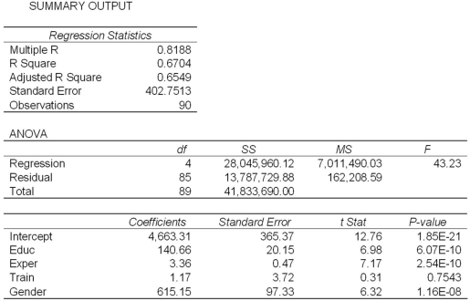 Model B: Salary = β0 + β1Educ + β2Exper + β3Gender + ε
 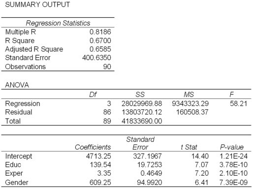 Refer to Exhibit 17.2.A group of female managers considers a discrimination lawsuit if on average their salaries can be statistically proven to be lower by more than $500 than the salaries of their male peers with the same level of education and experience.Using Model B,what is the alternative hypothesis for testing the lawsuit condition?
(Multiple Choice)
4.9/5 (41)
Exhibit 17.8.A realtor wants to predict and compare the prices of homes in three neighboring locations.She considers the following linear models:
Model A: Price = β0 + β1Size + β2Age + ε,
Model B: Price = β0 + β1Size + β2Loc1 + β3Loc2 + ε,
Model C: Price = β0 + β1Size + β2Age + β3Loc1 + β4Loc2 + ε,
where,
Price = the price of a home (in $thousands),
Size = the square footage (in square feet),
Loc1 = a dummy variable taking on 1 for Location 1,and 0 otherwise,
Loc2 = a dummy variable taking on 1 for Location 2,and 0 otherwise.
After collecting data on 52 sales and applying regression,her findings were summarized in the following table.
(Essay)
4.9/5 (31)
Exhibit 17.9.A bank manager is interested in assigning a rating to the holders of credit cards issued by her bank.The rating is based on the probability of defaulting on credit cards and is as follows.
(Essay)
4.8/5 (35)
Exhibit 17.9.A bank manager is interested in assigning a rating to the holders of credit cards issued by her bank.The rating is based on the probability of defaulting on credit cards and is as follows.  To estimate this probability,she decided to use the logistic model:
  ,
where,
y = a binary response variable with value 1 corresponding to a default,and 0 to a no default,
x1 = the ratio of the credit card balance to the credit card limit (in percent),
x2 = the ratio of the total debt to the annual income (in percent).
Using Minitab on the sample data,she arrived at the following estimates:
,
where,
y = a binary response variable with value 1 corresponding to a default,and 0 to a no default,
x1 = the ratio of the credit card balance to the credit card limit (in percent),
x2 = the ratio of the total debt to the annual income (in percent).
Using Minitab on the sample data,she arrived at the following estimates: 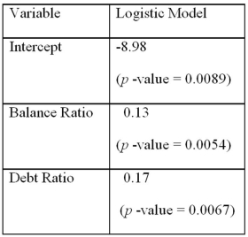 Note: The p-values of the corresponding tests are shown in parentheses below the estimated coefficients.
Refer to Exhibit 17.9.Assuming the debt ratio 30%,compute the increase in the probability of defaulting when the balance ratio goes up from 5% to 15%.
Note: The p-values of the corresponding tests are shown in parentheses below the estimated coefficients.
Refer to Exhibit 17.9.Assuming the debt ratio 30%,compute the increase in the probability of defaulting when the balance ratio goes up from 5% to 15%.
(Short Answer)
4.9/5 (39)
Exhibit 17.9.A bank manager is interested in assigning a rating to the holders of credit cards issued by her bank.The rating is based on the probability of defaulting on credit cards and is as follows.  To estimate this probability,she decided to use the logistic model:
 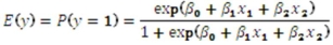 ,
where,
y = a binary response variable with value 1 corresponding to a default,and 0 to a no default,
x1 = the ratio of the credit card balance to the credit card limit (in percent),
x2 = the ratio of the total debt to the annual income (in percent).
Using Minitab on the sample data,she arrived at the following estimates:
,
where,
y = a binary response variable with value 1 corresponding to a default,and 0 to a no default,
x1 = the ratio of the credit card balance to the credit card limit (in percent),
x2 = the ratio of the total debt to the annual income (in percent).
Using Minitab on the sample data,she arrived at the following estimates:  Note: The p-values of the corresponding tests are shown in parentheses below the estimated coefficients.
Refer to Exhibits 17.9.Bob has a balance ratio of 10%,an annual income of $80,000,and $15,000 in total debt.Only applicants with excellent and good ratings are qualified for a loan.Find the maximum amount of loan Bob can get if he is required to maintain his excellent or good rating after getting this amount.
Note: The p-values of the corresponding tests are shown in parentheses below the estimated coefficients.
Refer to Exhibits 17.9.Bob has a balance ratio of 10%,an annual income of $80,000,and $15,000 in total debt.Only applicants with excellent and good ratings are qualified for a loan.Find the maximum amount of loan Bob can get if he is required to maintain his excellent or good rating after getting this amount.
(Short Answer)
5.0/5 (42)
For a linear regression model with a dummy variable d and an interaction variable xd,we:
(Multiple Choice)
4.7/5 (35)
Exhibit 17.8.A realtor wants to predict and compare the prices of homes in three neighboring locations.She considers the following linear models:
Model A: Price = β0 + β1Size + β2Age + ε,
Model B: Price = β0 + β1Size + β2Loc1 + β3Loc2 + ε,
Model C: Price = β0 + β1Size + β2Age + β3Loc1 + β4Loc2 + ε,
where,
Price = the price of a home (in $thousands),
Size = the square footage (in square feet),
Loc1 = a dummy variable taking on 1 for Location 1,and 0 otherwise,
Loc2 = a dummy variable taking on 1 for Location 2,and 0 otherwise.
After collecting data on 52 sales and applying regression,her findings were summarized in the following table. 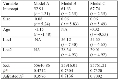 Note: The values of relevant test statistics are shown in parentheses below the estimated coefficients.
Refer to Exhibit 17.8.Using Model C,what is the conclusion for testing the joint significance of the two dummy variables at the 1% significance level?
Note: The values of relevant test statistics are shown in parentheses below the estimated coefficients.
Refer to Exhibit 17.8.Using Model C,what is the conclusion for testing the joint significance of the two dummy variables at the 1% significance level?
(Essay)
4.8/5 (34)
Exhibit 17.7.To examine the differences between salaries of male and female middle managers of a large bank,90 individuals were randomly selected and the following variables considered:
Salary = the monthly salary (excluding fringe benefits and bonuses),
Educ = the number of years of education,
Exper = the number of months of experience,
Gender = the gender of an individual;1 for males,and 0 for females.
The regression results for the models,
Model A: Salary = β0 + β1Educ + β2Exper + β3Gender + β4Exper × Gender + ε,
Model B: Salary = β0 + β1Educ + β2Exper + ε,are summarized below. 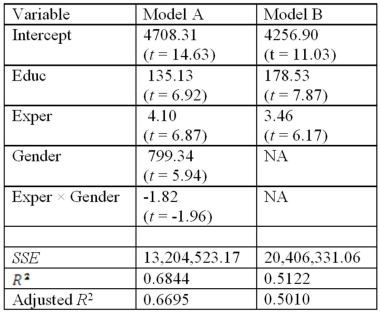 Note.The values of relevant test statistics are shown in parentheses below the estimated coefficients.
Refer to Exhibit 17.7.What is the value of the test statistic for testing the joint significance of Exper and Exper × Gender in Model A?
Note.The values of relevant test statistics are shown in parentheses below the estimated coefficients.
Refer to Exhibit 17.7.What is the value of the test statistic for testing the joint significance of Exper and Exper × Gender in Model A?
(Essay)
4.9/5 (42)
If the number of dummy variables representing a qualitative variable equals the number of categories of this variable,one deals with the problem of perfect multicollinearity.
(True/False)
4.9/5 (33)
Exhibit 17.9.A bank manager is interested in assigning a rating to the holders of credit cards issued by her bank.The rating is based on the probability of defaulting on credit cards and is as follows. 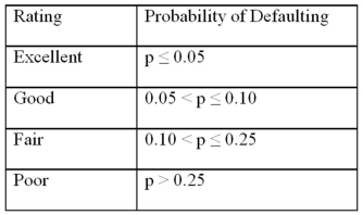 To estimate this probability,she decided to use the logistic model:
 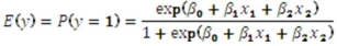 ,
where,
y = a binary response variable with value 1 corresponding to a default,and 0 to a no default,
x1 = the ratio of the credit card balance to the credit card limit (in percent),
x2 = the ratio of the total debt to the annual income (in percent).
Using Minitab on the sample data,she arrived at the following estimates:
,
where,
y = a binary response variable with value 1 corresponding to a default,and 0 to a no default,
x1 = the ratio of the credit card balance to the credit card limit (in percent),
x2 = the ratio of the total debt to the annual income (in percent).
Using Minitab on the sample data,she arrived at the following estimates:  Note: The p-values of the corresponding tests are shown in parentheses below the estimated coefficients.
Refer to Exhibit 17.9.What is the estimated logistic model?
Note: The p-values of the corresponding tests are shown in parentheses below the estimated coefficients.
Refer to Exhibit 17.9.What is the estimated logistic model?
(Essay)
4.8/5 (44)
Exhibit 17.8.A realtor wants to predict and compare the prices of homes in three neighboring locations.She considers the following linear models:
Model A: Price = β0 + β1Size + β2Age + ε,
Model B: Price = β0 + β1Size + β2Loc1 + β3Loc2 + ε,
Model C: Price = β0 + β1Size + β2Age + β3Loc1 + β4Loc2 + ε,
where,
Price = the price of a home (in $thousands),
Size = the square footage (in square feet),
Loc1 = a dummy variable taking on 1 for Location 1,and 0 otherwise,
Loc2 = a dummy variable taking on 1 for Location 2,and 0 otherwise.
After collecting data on 52 sales and applying regression,her findings were summarized in the following table.
(Essay)
4.8/5 (40)
Exhibit 17.5.An over-the-counter drug manufacturer wants to examine the effectiveness of a new drug in curing an illness most commonly in older patients.Thirteen patients are given the new drug and 13 patients are given the old drug.To avoid bias in the experiment,they are not told which drug is given to them.To check how the effectiveness depends on the age of patients,the following data has been collected. 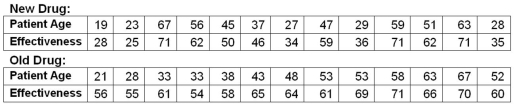 Assuming the variables: Effectiveness = the response variable measured on a scale from 0 to 100,
Age = the age of a patient (in years),
Drug = a binary variable with 1 for the new drug,and 0 for the old drug,the regression model,
Effectiveness = β0 + β1Age + β2Drug + β3Age × Drug,is considered,and the following Excel results are available:
Assuming the variables: Effectiveness = the response variable measured on a scale from 0 to 100,
Age = the age of a patient (in years),
Drug = a binary variable with 1 for the new drug,and 0 for the old drug,the regression model,
Effectiveness = β0 + β1Age + β2Drug + β3Age × Drug,is considered,and the following Excel results are available: 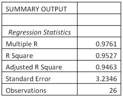
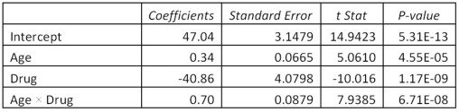 Refer to Exhibit 17.5.Which of the following is true?
(Multiple Choice)
5.0/5 (32)
Filters
- Essay(0)
- Multiple Choice(0)
- Short Answer(0)
- True False(0)
- Matching(0)