Exam 17: Regression Models With Dummy Variables

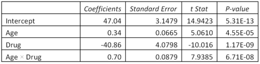
Exhibit 17.5.An over-the-counter drug manufacturer wants to examine the effectiveness of a new drug in curing an illness most commonly in older patients.Thirteen patients are given the new drug and 13 patients are given the old drug.To avoid bias in the experiment,they are not told which drug is given to them.To check how the effectiveness depends on the age of patients,the following data has been collected. Assuming the variables: Effectiveness = the response variable measured on a scale from 0 to 100, Age = the age of a patient (in years), Drug = a binary variable with 1 for the new drug,and 0 for the old drug,the regression model, Effectiveness = β₀ + β₁Age + β₂Drug + β₃Age × Drug,is considered,and the following Excel results are available: 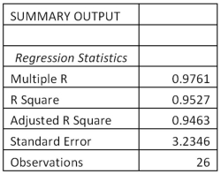Refer to Exhibit 17.5.What is the predicted effectiveness of the new drug for a 62 years old patient?

In the regression equation 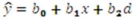,a dummy variable d affects the slope of the line.

Exhibit 17.5.An over-the-counter drug manufacturer wants to examine the effectiveness of a new drug in curing an illness most commonly in older patients.Thirteen patients are given the new drug and 13 patients are given the old drug.To avoid bias in the experiment,they are not told which drug is given to them.To check how the effectiveness depends on the age of patients,the following data has been collected. Assuming the variables: Effectiveness = the response variable measured on a scale from 0 to 100, Age = the age of a patient (in years), Drug = a binary variable with 1 for the new drug,and 0 for the old drug,the regression model, Effectiveness = β₀ + β₁Age + β₂Drug + β₃Age × Drug,is considered,and the following Excel results are available: Refer to Exhibit 17.5.What is the estimated regression model for the old drug?

Which of the following variables is not qualitative?

Exhibit 17.8.A realtor wants to predict and compare the prices of homes in three neighboring locations.She considers the following linear models: Model A: Price = β₀ + β₁Size + β₂Age + ε, Model B: Price = β₀ + β₁Size + β₂Loc1 + β₃Loc2 + ε, Model C: Price = β₀ + β₁Size + β₂Age + β₃Loc1 + β₄Loc2 + ε, where, Price = the price of a home (in $thousands), Size = the square footage (in square feet), Loc1 = a dummy variable taking on 1 for Location 1,and 0 otherwise, Loc2 = a dummy variable taking on 1 for Location 2,and 0 otherwise. After collecting data on 52 sales and applying regression,her findings were summarized in the following table. Note: The values of relevant test statistics are shown in parentheses below the estimated coefficients. Refer to Exhibit 17.8.What is regression equation for model B?

Exhibit 17.8.A realtor wants to predict and compare the prices of homes in three neighboring locations.She considers the following linear models: Model A: Price = β₀ + β₁Size + β₂Age + ε, Model B: Price = β₀ + β₁Size + β₂Loc1 + β₃Loc2 + ε, Model C: Price = β₀ + β₁Size + β₂Age + β₃Loc1 + β₄Loc2 + ε, where, Price = the price of a home (in $thousands), Size = the square footage (in square feet), Loc1 = a dummy variable taking on 1 for Location 1,and 0 otherwise, Loc2 = a dummy variable taking on 1 for Location 2,and 0 otherwise. After collecting data on 52 sales and applying regression,her findings were summarized in the following table. Note: The values of relevant test statistics are shown in parentheses below the estimated coefficients. Refer to Exhibit 17.8.Using Model B,what is the predicted price of a 2,500 square feet home in Location 1?

Exhibit 17.9.A bank manager is interested in assigning a rating to the holders of credit cards issued by her bank.The rating is based on the probability of defaulting on credit cards and is as follows. 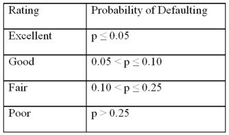To estimate this probability,she decided to use the logistic model: 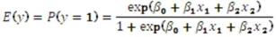, where, y = a binary response variable with value 1 corresponding to a default,and 0 to a no default, x₁ = the ratio of the credit card balance to the credit card limit (in percent), x₂ = the ratio of the total debt to the annual income (in percent). Using Minitab on the sample data,she arrived at the following estimates: 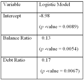Note: The p-values of the corresponding tests are shown in parentheses below the estimated coefficients. Refer to Exhibits 17.9.What will be the rating for a person with a balance ratio of 15% and a debt ratio of 30%?

Exhibit 17.2.To examine the differences between salaries of male and female middle managers of a large bank,90 individuals were randomly selected and the following variables considered: Salary = the monthly salary (excluding fringe benefits and bonuses), Educ = the number of years of education, Exper = the number of months of experience, Train = the number of weeks of training, Gender = the gender of an individual;1 for males,and 0 for females. Also,the following Excel partial outputs corresponding to the following models are available: Model A: Salary = β₀ + β₁Educ + β₂Exper + β₃Train + β₄Gender + ε 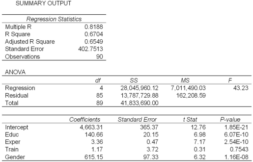Model B: Salary = β₀ + β₁Educ + β₂Exper + β₃Gender + ε Refer to Exhibit 17.2.Using Model B,what is the regression equation found by Excel for males?

Consider the model y = β₀ + β₁x + β₂d + ε,where x is a quantitative variable and d is a dummy variable.For d = 1,the predicted value of y is computed as:

Exhibit 17.3.Consider the regression model, Humidity = β₀ + β₁Temperature + β₂Spring + β₃Summer + β₄Fall + β₅Rain + ε, Where the dummy variables Spring,Summer,and Fall represent the qualitative variable Season (spring,summer,fall,winter),and the dummy variable Rain is defined as Rain = 1 if rainy day,Rain = 0 otherwise. Refer to Exhibit 17.3.What is the regression equation for the winter days?

For the linear probability model y = β₀ + β₁x + ε,the predictions made by can be always interpreted as probabilities.

Exhibit 17.2.To examine the differences between salaries of male and female middle managers of a large bank,90 individuals were randomly selected and the following variables considered: Salary = the monthly salary (excluding fringe benefits and bonuses), Educ = the number of years of education, Exper = the number of months of experience, Train = the number of weeks of training, Gender = the gender of an individual;1 for males,and 0 for females. Also,the following Excel partial outputs corresponding to the following models are available: Model A: Salary = β₀ + β₁Educ + β₂Exper + β₃Train + β₄Gender + ε Model B: Salary = β₀ + β₁Educ + β₂Exper + β₃Gender + ε Refer to Exhibit 17.2.Using Model A,what is the estimated average difference between the salaries of male and female employees with the same years of education,months of experience,and weeks of training?

In the regression equation = b₀ + b₁x + b₂dx with a dummy variable d,when d changes from 0 to 1,the change in the slope of the corresponding lines is given by:

A logistic model can be estimated with the method of:

Exhibit 17.1.A researcher has developed the following regression equation to predict the prices of luxurious Oceanside condominium units, , where Price = the price of a unit (in $thousands), Size = the square footage (in square feet), View = a dummy variable taking on 1 for an ocean view unit,and 0 for a bay view unit. Refer to Exhibit 17.1.What is the predicted difference in prices of the ocean view and bay view units with the same square footage?

Exhibit 17.2.To examine the differences between salaries of male and female middle managers of a large bank,90 individuals were randomly selected and the following variables considered: Salary = the monthly salary (excluding fringe benefits and bonuses), Educ = the number of years of education, Exper = the number of months of experience, Train = the number of weeks of training, Gender = the gender of an individual;1 for males,and 0 for females. Also,the following Excel partial outputs corresponding to the following models are available: Model A: Salary = β₀ + β₁Educ + β₂Exper + β₃Train + β₄Gender + ε Model B: Salary = β₀ + β₁Educ + β₂Exper + β₃Gender + ε 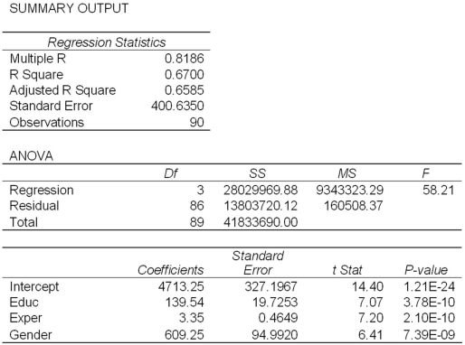Refer to Exhibit 17.2.Under the assumption of the same years of education and months of experience,what is the p-value for testing whether the mean salary of males is greater than the mean salary of females using Model B?

Exhibit 17.8.A realtor wants to predict and compare the prices of homes in three neighboring locations.She considers the following linear models: Model A: Price = β₀ + β₁Size + β₂Age + ε, Model B: Price = β₀ + β₁Size + β₂Loc1 + β₃Loc2 + ε, Model C: Price = β₀ + β₁Size + β₂Age + β₃Loc1 + β₄Loc2 + ε, where, Price = the price of a home (in $thousands), Size = the square footage (in square feet), Loc1 = a dummy variable taking on 1 for Location 1,and 0 otherwise, Loc2 = a dummy variable taking on 1 for Location 2,and 0 otherwise. After collecting data on 52 sales and applying regression,her findings were summarized in the following table. 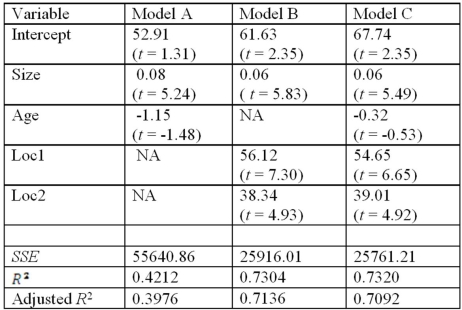Note: The values of relevant test statistics are shown in parentheses below the estimated coefficients. Refer to Exhibit 17.8.Using Model B,what is the predicted difference between the price of homes with the same square footage located in Location 2 and Location 3?

Exhibit 17.9.A bank manager is interested in assigning a rating to the holders of credit cards issued by her bank.The rating is based on the probability of defaulting on credit cards and is as follows.

A model y = β₀ + β₁x + ε,in which y is a binary variable,is called a linear probability model.

Which of the following regression models does not include an interaction variable?