Exam 17: Regression Models With Dummy Variables

The major advantage of a logistic model over the corresponding linear probability model is that the predicted values of y are always between:

Consider the regression equation = b₀ + b₁xd with b₁ > 0 and a dummy variable d.If d changes from 0 to 1,which of the following is true?

Exhibit 17.8.A realtor wants to predict and compare the prices of homes in three neighboring locations.She considers the following linear models: Model A: Price = β₀ + β₁Size + β₂Age + ε, Model B: Price = β₀ + β₁Size + β₂Loc1 + β₃Loc2 + ε, Model C: Price = β₀ + β₁Size + β₂Age + β₃Loc1 + β₄Loc2 + ε, where, Price = the price of a home (in $thousands), Size = the square footage (in square feet), Loc1 = a dummy variable taking on 1 for Location 1,and 0 otherwise, Loc2 = a dummy variable taking on 1 for Location 2,and 0 otherwise. After collecting data on 52 sales and applying regression,her findings were summarized in the following table.

Exhibit 17.9.A bank manager is interested in assigning a rating to the holders of credit cards issued by her bank.The rating is based on the probability of defaulting on credit cards and is as follows. 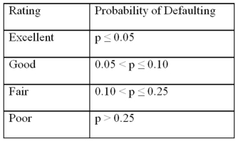To estimate this probability,she decided to use the logistic model: 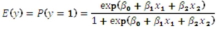, where, y = a binary response variable with value 1 corresponding to a default,and 0 to a no default, x₁ = the ratio of the credit card balance to the credit card limit (in percent), x₂ = the ratio of the total debt to the annual income (in percent). Using Minitab on the sample data,she arrived at the following estimates: 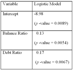Note: The p-values of the corresponding tests are shown in parentheses below the estimated coefficients. Refer to Exhibits 17.9.Assuming the debt ratio is 30%,what is the range of values for the balance ratio that yields the fair rating?

Exhibit 17.3.Consider the regression model, Humidity = β₀ + β₁Temperature + β₂Spring + β₃Summer + β₄Fall + β₅Rain + ε, Where the dummy variables Spring,Summer,and Fall represent the qualitative variable Season (spring,summer,fall,winter),and the dummy variable Rain is defined as Rain = 1 if rainy day,Rain = 0 otherwise. Refer to Exhibit 17.3.What is the regression equation for the summer rainy days?

Exhibit 17.4.A researcher wants to examine how the remaining balance on $100,000 loans taken 10-20 years ago depends on whether the loan was a prime or sub-prime loan.He collected a sample of 25 prime loans and 25 sub-prime loans and records the data in the following variables: Balance = the remaining amount of loan to be paid off (in dollars), Time = the time elapsed from taking the loan, Prime = a dummy variable assuming 1 for prime loans,and 0 for sub-prime loans. The regression results obtained for the models: Model A: Balance = β₀ + β₁Prime + ε Model B: Balance = β₀ + β₁Time + β₂Prime + β₃Time × Prime + ε Model C: Balance = β₀ + β₁Prime + β₂Time × Prime + ε, Are summarized below. Note.The values of relevant test statistics are shown in parentheses below the estimated coefficients. Refer to Exhibit 17.4.Which of the three models would you choose to make the predictions of the remaining loan balance?

For the model y = β₀ + β₁x + β₂d + ε,which test is used for testing the significance of a dummy variable d?

The model y = β₀ + β₁x + β₂d + β₃xd + ε is an example of a:

A dummy variable is a variable that takes on the values of 0 and 1.

Exhibit 17.3.Consider the regression model, Humidity = β₀ + β₁Temperature + β₂Spring + β₃Summer + β₄Fall + β₅Rain + ε, Where the dummy variables Spring,Summer,and Fall represent the qualitative variable Season (spring,summer,fall,winter),and the dummy variable Rain is defined as Rain = 1 if rainy day,Rain = 0 otherwise. Refer to Exhibit 17.3.Assuming the same temperature and precipitation condition,what is the difference between the predicted humidity for summer and fall days?

For the model y = β₀ + β₁x + β₂d₁ + β₃d₂ + ε,which test is used for testing the joint significance of the dummy variables d₁ and d₂?

Exhibit 17.2.To examine the differences between salaries of male and female middle managers of a large bank,90 individuals were randomly selected and the following variables considered: Salary = the monthly salary (excluding fringe benefits and bonuses), Educ = the number of years of education, Exper = the number of months of experience, Train = the number of weeks of training, Gender = the gender of an individual;1 for males,and 0 for females. Also,the following Excel partial outputs corresponding to the following models are available: Model A: Salary = β₀ + β₁Educ + β₂Exper + β₃Train + β₄Gender + ε 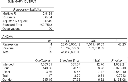Model B: Salary = β₀ + β₁Educ + β₂Exper + β₃Gender + ε Refer to Exhibit 17.2.Under the assumption of the same years of education and months of experience,what is the null hypothesis for testing whether the mean salary of males is greater than the mean salary of females using Model B?

Exhibit 17.2.To examine the differences between salaries of male and female middle managers of a large bank,90 individuals were randomly selected and the following variables considered: Salary = the monthly salary (excluding fringe benefits and bonuses), Educ = the number of years of education, Exper = the number of months of experience, Train = the number of weeks of training, Gender = the gender of an individual;1 for males,and 0 for females. Also,the following Excel partial outputs corresponding to the following models are available: Model A: Salary = β₀ + β₁Educ + β₂Exper + β₃Train + β₄Gender + ε Model B: Salary = β₀ + β₁Educ + β₂Exper + β₃Gender + ε Refer to Exhibit 17.2.What is the regression equation found by Excel for Model A?

Exhibit 17.2.To examine the differences between salaries of male and female middle managers of a large bank,90 individuals were randomly selected and the following variables considered: Salary = the monthly salary (excluding fringe benefits and bonuses), Educ = the number of years of education, Exper = the number of months of experience, Train = the number of weeks of training, Gender = the gender of an individual;1 for males,and 0 for females. Also,the following Excel partial outputs corresponding to the following models are available: Model A: Salary = β₀ + β₁Educ + β₂Exper + β₃Train + β₄Gender + ε Model B: Salary = β₀ + β₁Educ + β₂Exper + β₃Gender + ε Refer to Exhibit 17.2.When testing the individual significance of Train in Model A,what is the test conclusion at 10% significance level?

Exhibit 17.4.A researcher wants to examine how the remaining balance on $100,000 loans taken 10-20 years ago depends on whether the loan was a prime or sub-prime loan.He collected a sample of 25 prime loans and 25 sub-prime loans and records the data in the following variables: Balance = the remaining amount of loan to be paid off (in dollars), Time = the time elapsed from taking the loan, Prime = a dummy variable assuming 1 for prime loans,and 0 for sub-prime loans. The regression results obtained for the models: Model A: Balance = β₀ + β₁Prime + ε Model B: Balance = β₀ + β₁Time + β₂Prime + β₃Time × Prime + ε Model C: Balance = β₀ + β₁Prime + β₂Time × Prime + ε, Are summarized below. Note.The values of relevant test statistics are shown in parentheses below the estimated coefficients. Refer to Exhibit 17.4.Using Model C,what is the predicted balance on a $100,000 prime loan taken 15 years ago?

Exhibit 17.2.To examine the differences between salaries of male and female middle managers of a large bank,90 individuals were randomly selected and the following variables considered: Salary = the monthly salary (excluding fringe benefits and bonuses), Educ = the number of years of education, Exper = the number of months of experience, Train = the number of weeks of training, Gender = the gender of an individual;1 for males,and 0 for females. Also,the following Excel partial outputs corresponding to the following models are available: Model A: Salary = β₀ + β₁Educ + β₂Exper + β₃Train + β₄Gender + ε Model B: Salary = β₀ + β₁Educ + β₂Exper + β₃Gender + ε 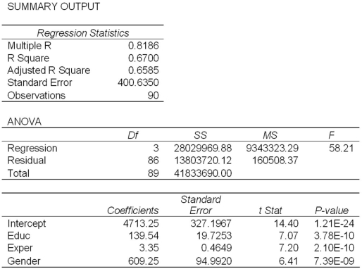Refer to Exhibit 17.2.A group of female managers considers a discrimination lawsuit if on average their salaries could be statistically proven to be lower by more than $500 than the salaries of their male peers with the same level of education and experience.Using Model B,what is the conclusion of the appropriate test at 10% significance level?

Regression models that use a binary variable as the response variable are called binary choice models.

For the model y = β₀ + β₁x + β₂xd + ε,what are the hypotheses for testing the individual significance of the interaction variable xd?

The major shortcoming of the general linear probability model y = β₀ + β₁x₁ + β₂x₂ + ∙∙∙+ β_kx_1k + ε,is that the predicted values of y can be sometimes

Exhibit 17.4.A researcher wants to examine how the remaining balance on $100,000 loans taken 10-20 years ago depends on whether the loan was a prime or sub-prime loan.He collected a sample of 25 prime loans and 25 sub-prime loans and records the data in the following variables: Balance = the remaining amount of loan to be paid off (in dollars), Time = the time elapsed from taking the loan, Prime = a dummy variable assuming 1 for prime loans,and 0 for sub-prime loans. The regression results obtained for the models: Model A: Balance = β₀ + β₁Prime + ε Model B: Balance = β₀ + β₁Time + β₂Prime + β₃Time × Prime + ε Model C: Balance = β₀ + β₁Prime + β₂Time × Prime + ε, Are summarized below. 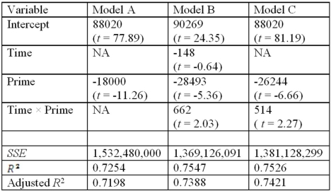Note.The values of relevant test statistics are shown in parentheses below the estimated coefficients. Refer to Exhibit 17.4.What is the p-value for testing the significance of Time in Model B?