Exam 20: Model Building

A traffic consultant has analysed the factors that affect the number of traffic fatalities. She has come to the conclusion that two important variables are the number of cars and the number of tractor-trailer trucks. She proposed the second-order model with interaction: $y =$ $\beta _ { 0 } + \beta _ { 1 } x _ { 1 } + \beta _ { 2 } x _ { 2 } + \beta _ { 3 } x _ { 1 } ^ { 2 } + \beta _ { 4 } x _ { 2 } ^ { 2 } + \beta _ { 5 } x _ { 1 } x _ { 2 } + \varepsilon$ . Where: y = number of annual fatalities per shire. $x _ { 1 }$ = number of cars registered in the shire (in units of 10 000). $x _ { 2 }$ = number of trucks registered in the shire (in units of 1000). The computer output (based on a random sample of 35 shires) is shown below. THE REGRESSION EQUATION IS $y =$ $69.7 + 11.3 x _ { 1 } + 7.61 x _ { 2 } - 1.15 x _ { 1 } ^ { 2 } - 0.51 x _ { 2 } ^ { 2 } - 0.13 x _ { 1 } x _ { 2 }$ . Predictor Coef SDev T Constant 69.7 41.3 1.688 11.3 5.1 2.216 7.61 2.55 2.984 -1.15 0.64 -1.797 -0.51 0.20 -2.55 -0.13 0.10 -1.30 S = 15.2 R-Sq = 47.2%. ANALYSIS OF VARIANCE Source of df SS MS F Variation Regression 5 5959 1191.800 5.181 Error 29 6671 230.034 Total 34 12630 What does the coefficient of $x _ { 2 } ^ { 2 }$ tell you about the model?

An avid football fan was in the process of examining the factors that determine the success or failure of football teams. He noticed that teams with many rookies and teams with many veterans seem to do quite poorly. To further analyse his beliefs, he took a random sample of 20 teams and proposed a second-order model with one independent variable. The selected model is: $y = \beta _ { 0 } + \beta _ { 1 } x + \beta _ { 2 } x ^ { 2 } + \varepsilon$ . where y = winning team's percentage. x = average years of professional experience. The computer output is shown below: THE REGRESSION EQUATION IS: $y =$ $32.6 + 5.96 x - 0.48 x ^ { 2 }$ Predictor Coef S2Dev T Constant 32.6 19.3 1.689 x 5.96 2.41 2.473 -0.48 0.22 -2.182 S = 16.1 R-Sq = 43.9%. ANALYSIS OF VARIANCE Source of Variation df SS MS F Regression 2 3452 1726 6.663 Error 17 4404 259.059 Total 19 7856 What is the coefficient of determination? Explain what this statistic tells you about the model.

Consider the following data for two variables, x and y. x 7 10 3 5 3 10 4 14 5 8 y 35.0 28.5 45.0 45.0 55.0 25.0 37.5 27.5 30.0 27.5 Use the model in = 66.799 -7.307x + 0.324x² to predict the value of y when x = 10.

Consider the following data for two variables, x and y. x 7 10 3 5 3 10 4 14 5 8 y 35.0 28.5 45.0 45.0 55.0 25.0 37.5 27.5 30.0 27.5 Use Excel to develop a scatter diagram for the data. Does the scatter diagram suggest an estimated regression equation of the form ŷ = b₀ +b₁x + b₂x²? Explain.

A first-order model was used in a regression analysis involving 25 observations to study the relationship between a dependent variable y and three independent variables, $x _ { 1 }$ , $x _ { 2 }$ and $X _ { 3 }$ . The analysis showed that the mean squares for regression is 160 and the sum of squares for error is 1050. In addition, the following is a partial computer printout. Predictor Coef StDev Constant 25 4 18 6 -12 4.8 6 5 Is there sufficient evidence at the 5% significance level to indicate that $X _ { 3 }$ is positively linearly related to y?

Suppose that the sample regression line of a first order model is $= 8 + 2 x _ { 1 } + 3 x _ { 2 }$ . If we examine the relationship between y and $x _ { 1 }$ for four different values of $x _ { 2 }$ , we observe that the:

An economist is in the process of developing a model to predict the price of gold. She believes that the two most important variables are the price of a barrel of oil $\left( x _ { 1 } \right)$ and the interest rate $\left( x _ { 2 } \right)$ She proposes the first-order model with interaction: $y = \beta _ { 0 } + \beta _ { 1 } x _ { 1 } + \beta _ { 2 } x _ { 2 } + \beta _ { 3 } x _ { 1 } x _ { 3 } + \varepsilon$ . A random sample of 20 daily observations was taken. The computer output is shown below. THE REGRESSION EQUATION IS $y =$ $115.6 + 22.3 x _ { 1 } + 14.7 x _ { 2 } - 1.36 x _ { 1 } x _ { 2 }$ . Predictor Coef StDev T Constant 115.6 78.1 1.480 22.3 7.1 3.141 14.7 6.3 2.333 -1.36 0.52 -2.615 S = 20.9 R-Sq = 55.4%. ANALYSIS OF VARIANCE Source of Variation df SS MS F Regression 3 8661 2887.0 6.626 Error 16 6971 435.7 Total 19 15632 Interpret the coefficient $b _ { 1 }$ .

A first-order model was used in a regression analysis involving 25 observations to study the relationship between a dependent variable y and three independent variables, $x _ { 1 }$ , $x _ { 2 }$ and $X _ { 3 }$ . The analysis showed that the mean squares for regression is 160 and the sum of squares for error is 1050. In addition, the following is a partial computer printout. Predictor Coef StDev Constant 25 4 18 6 -12 4.8 6 5 Develop the ANOVA table.

In a stepwise regression procedure, if two independent variables are highly correlated, then one variable usually eliminates the second variable.

The owner of an air conditioner business wants to investigate the relationship between the weekly number of air conditioners sold, temperature and the seasons of the year. A random sample of 14 weeks is taken, with the average temperature of that week (in degrees Celsius) and the quarter from which that week belonged, noted. There are three indicator variables, March, September and December. Excel is used to generate the following multiple linear regression output. Using the p-values from Excel, state which of the quarters are statistically significant at α of 5%.

In a first-order model with two predictors, $x _ { 1 }$ and $x _ { 2 }$ , an interaction term may be used when the relationship between the dependent variable $y$ and the predictor variables is linear.

The owner of an air conditioner business wants to investigate the relationship between the weekly number of air conditioners sold with average weekly temperature and the seasons of the year. A random sample of 14 weeks is taken, with the average temperature of that week (in degrees Celsius) and the quarter from which that week belonged, noted. There are three indicator variables: March, September and December. Excel is used to generate the following multiple linear regression output. Test the significance of the coefficient of Temperature, at the 5% level of α. Justify your choice of the alternative hypothesis.

The owner of an air conditioner business wants to investigate the relationship between the weekly number of air conditioners sold, temperature and the seasons of the year. A random sample of 14 weeks is taken, with the average temperature of that week (in degrees Celsius) and the quarter from which that week belonged, noted. There are three indicator variables, March, September and December. Excel is used to generate the following multiple linear regression output. 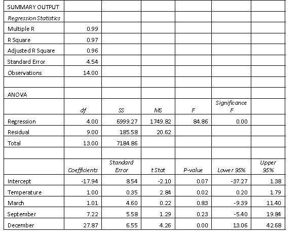(a) Write the linear regression model for each quarter: March, June, September and December (a) Roughly, sketch on the same set of axes, showing the intercept and the slope.

A first-order model was used in a regression analysis involving 25 observations to study the relationship between a dependent variable y and three independent variables, $x _ { 1 }$ , $x _ { 2 }$ and $X _ { 3 }$ . The analysis showed that the mean squares for regression is 160 and the sum of squares for error is 1050. In addition, the following is a partial computer printout. Predictor Coef StDev Constant 25 4 18 6 -12 4.8 6 5 Test at the 5% significance level to determine whether $x _ { 1 }$ is linearly related to y.

In explaining students' test scores, which of the following independent variables would not be adequately represented by an indicator variable?

An avid football fan was in the process of examining the factors that determine the success or failure of football teams. He noticed that teams with many rookies and teams with many veterans seem to do quite poorly. To further analyse his beliefs, he took a random sample of 20 teams and proposed a second-order model with one independent variable. The selected model is: $y = \beta _ { 0 } + \beta _ { 1 } x + \beta _ { 2 } x ^ { 2 } + \varepsilon$ . where y = winning team's percentage. x = average years of professional experience. The computer output is shown below: THE REGRESSION EQUATION IS: $y =$ $32.6 + 5.96 x - 0.48 x ^ { 2 }$ Predictor Coef S2Dev T Constant 32.6 19.3 1.689 x 5.96 2.41 2.473 -0.48 0.22 -2.182 S = 16.1 R-Sq = 43.9%. ANALYSIS OF VARIANCE Source of Variation df SS MS F Regression 2 3452 1726 6.663 Error 17 4404 259.059 Total 19 7856 Test to determine at the 10% significance level if the linear term should be retained.

Regression analysis allows the statistics practitioner to use mathematical models to realistically describe relationships between the dependent variable and independent variables.

When we plot x versus y, the graph of the model $y = \beta _ { 0 } + \beta _ { 1 } x + \beta _ { 2 } x ^ { 2 }$ + $\varepsilon$ is shaped like a:

A traffic consultant has analysed the factors that affect the number of traffic fatalities. She has come to the conclusion that two important variables are the number of cars and the number of tractor-trailer trucks. She proposed the second-order model with interaction: $y =$ $\beta _ { 0 } + \beta _ { 1 } x _ { 1 } + \beta _ { 2 } x _ { 2 } + \beta _ { 3 } x _ { 1 } ^ { 2 } + \beta _ { 4 } x _ { 2 } ^ { 2 } + \beta _ { 5 } x _ { 1 } x _ { 2 } + \varepsilon$ . Where: y = number of annual fatalities per shire. $x _ { 1 }$ = number of cars registered in the shire (in units of 10 000). $x _ { 2 }$ = number of trucks registered in the shire (in units of 1000). The computer output (based on a random sample of 35 shires) is shown below. THE REGRESSION EQUATION IS $y =$ $69.7 + 11.3 x _ { 1 } + 7.61 x _ { 2 } - 1.15 x _ { 1 } ^ { 2 } - 0.51 x _ { 2 } ^ { 2 } - 0.13 x _ { 1 } x _ { 2 }$ . Predictor Coef SDev T Constant 69.7 41.3 1.688 11.3 5.1 2.216 7.61 2.55 2.984 -1.15 0.64 -1.797 -0.51 0.20 -2.55 -0.13 0.10 -1.30 S = 15.2 R-Sq = 47.2%. ANALYSIS OF VARIANCE Source of df SS MS F Variation Regression 5 5959 1191.800 5.181 Error 29 6671 230.034 Total 34 12630 Test at the 1% significance level to determine whether the $x _ { 1 }$ term should be retained in the model.

A regression analysis involving 40 observations and five independent variables revealed that the total variation in the dependent variable y is 1080 and that the mean square for error is 30. Source of Variation df SS MS F Regression 5 60 12 0.40 Error 34 1020 30 Total 39 1080 Test the significance of the overall equation at the 5% level of significance.