Exam 20: Model Building

The model y = $\beta$ ₀ + $\beta$ ₁x + is referred to as a simple linear regression model.

The model $y = \beta _ { 0 } + \beta _ { 1 } x _ { 1 } + \beta _ { 2 } x _ { 2 } + \beta _ { 3 } x _ { 1 } x _ { 2 }$ + $\varepsilon$ is referred to as a:

An economist is analysing the incomes of professionals (physicians, dentists and lawyers). He realises that an important factor is the number of years of experience. However, he wants to know if there are differences among the three professional groups. He takes a random sample of 125 professionals and estimates the multiple regression model: $y = \beta _ { 0 } + \beta _ { 1 } x _ { 1 } + \beta _ { 2 } x _ { 2 } + \beta _ { 3 } x _ { 3 } + \varepsilon$ . where y = annual income (in $1000). $x _ { 1 }$ = years of experience. $x _ { 2 }$ = 1 if physician. = 0 if not. $X _ { 3 }$ = 1 if dentist. = 0 if not. The computer output is shown below. THE REGRESSION EQUATION IS $y =$ $71.65 + 2.07 x _ { 1 } + 10.16 x _ { 2 } - 7.44 x _ { 3 }$ . Predictor Coef SDev T Constant 71.65 18.56 3.860 2.07 0.81 2.556 10.16 3.16 3.215 -7.44 2.85 -2.611 S = 42.6 R-Sq = 30.9%. ANALYSIS OF VARIANCE Source of Variation df SS MS F Regression 3 98008 32669.333 18.008 Error 121 219508 1814.116 Total 124 317516 Is there enough evidence at the 10% significance level to conclude that dentists earn less on average than lawyers?

An economist is in the process of developing a model to predict the price of gold. She believes that the two most important variables are the price of a barrel of oil $\left( x _ { 1 } \right)$ and the interest rate $\left( x _ { 2 } \right)$ She proposes the first-order model with interaction: $y = \beta _ { 0 } + \beta _ { 1 } x _ { 1 } + \beta _ { 2 } x _ { 2 } + \beta _ { 3 } x _ { 1 } x _ { 3 } + \varepsilon$ . A random sample of 20 daily observations was taken. The computer output is shown below. THE REGRESSION EQUATION IS $y =$ $115.6 + 22.3 x _ { 1 } + 14.7 x _ { 2 } - 1.36 x _ { 1 } x _ { 2 }$ . Predictor Coef StDev T Constant 115.6 78.1 1.480 22.3 7.1 3.141 14.7 6.3 2.333 -1.36 0.52 -2.615 S = 20.9 R-Sq = 55.4%. ANALYSIS OF VARIANCE Source of Variation df SS MS F Regression 3 8661 2887.0 6.626 Error 16 6971 435.7 Total 19 15632 Do these results allow us at the 5% significance level to conclude that the model is useful in predicting the price of gold?

Suppose that the sample regression equation of a model is $= 4 + 1.5 x _ { 1 } + 2 x _ { 2 } - x _ { 1 } x _ { 2 }$ . If we examine the relationship between $x _ { 1 }$ and y for four different values of $x _ { 2 }$ , we observe that the four equations produced differ only in the intercept term.

In regression analysis, we can use 11 indicator variables to represent 12 months of the year.

The model $y = \beta _ { 0 } + \beta _ { 1 } x _ { 1 } + \beta _ { 2 } x _ { 2 }$ + $\varepsilon$ is referred to as a:

Suppose that the sample regression equation of a model is $= 10 + 4 x _ { 1 } + 3 x _ { 2 } - x _ { 1 } x _ { 2 }$ . If we examine the relationship between $x _ { 1 }$ and y for three different values of $x _ { 2 }$ , we observe that the:

Which of the following describes the numbers that an indicator variable can have in a regression model?

Stepwise regression is an iterative procedure that can only add one independent variable at a time.

A regression analysis was performed to study the relationship between a dependent variable and four independent variables. The following information was obtained: r² = 0.95, SSR = 9800, n = 50. Create the ANOVA table.

The owner of an air conditioner business wants to investigate the relationship between the weekly number of air conditioners sold, temperature and the seasons of the year. A random sample of 14 weeks is taken, with the average temperature of that week (in degrees Celsius) and the quarter from which that week belonged, noted. There are three indicator variables, March, September and December. Excel is used to generate the following multiple linear regression output. (a) Estimate the number of air conditioners sold in the first week of December, on a 40 degree Celsius day. Is this a good estimate? (b) If the actual number of air conditioners sold in the first week of December was 45 air conditioners, find the residual? Has the model over estimated or underestimated the weekly number of air conditioners sold by this business?

A regression analysis involving 40 observations and five independent variables revealed that the total variation in the dependent variable y is 1080 and that the mean square for error is 30. Create the ANOVA table.

Consider the following data for two variables, x and y. x 7 10 3 5 3 10 4 14 5 8 y 35.0 28.5 45.0 45.0 55.0 25.0 37.5 27.5 30.0 27.5 Use Excel to find the coefficient of determination. What does this statistic tell you about this simple linear model?

The owner of an air conditioner business wants to investigate the relationship between the weekly number of air conditioners sold, temperature and the seasons of the year. A random sample of 14 weeks is taken, with the average temperature of that week (in degrees Celsius) and the quarter from which that week belonged, noted. There are three indicator variables, March, September and December. Excel is used to generate the following multiple linear regression output. 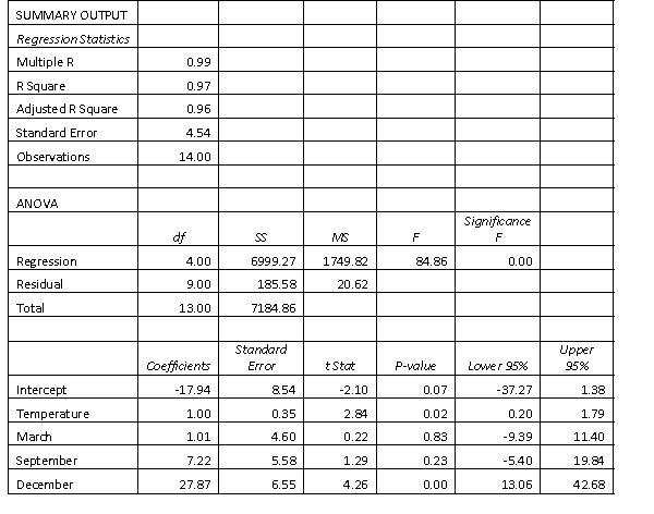Test the significance of the overall regression equation.

An economist is analysing the incomes of professionals (physicians, dentists and lawyers). He realises that an important factor is the number of years of experience. However, he wants to know if there are differences among the three professional groups. He takes a random sample of 125 professionals and estimates the multiple regression model: $y = \beta _ { 0 } + \beta _ { 1 } x _ { 1 } + \beta _ { 2 } x _ { 2 } + \beta _ { 3 } x _ { 3 } + \varepsilon$ . where y = annual income (in $1000). $x _ { 1 }$ = years of experience. $x _ { 2 }$ = 1 if physician. = 0 if not. $X _ { 3 }$ = 1 if dentist. = 0 if not. The computer output is shown below. THE REGRESSION EQUATION IS $y =$ $71.65 + 2.07 x _ { 1 } + 10.16 x _ { 2 } - 7.44 x _ { 3 }$ . Predictor Coef SDev T Constant 71.65 18.56 3.860 2.07 0.81 2.556 10.16 3.16 3.215 -7.44 2.85 -2.611 S = 42.6 R-Sq = 30.9%. ANALYSIS OF VARIANCE Source of Variation df SS MS F Regression 3 98008 32669.333 18.008 Error 121 219508 1814.116 Total 124 317516 Is there enough evidence at the1% significant level to conclude that physicians earn more on average than lawyers?

A traffic consultant has analysed the factors that affect the number of traffic fatalities. She has come to the conclusion that two important variables are the number of cars and the number of tractor-trailer trucks. She proposed the second-order model with interaction: $y =$ $\beta _ { 0 } + \beta _ { 1 } x _ { 1 } + \beta _ { 2 } x _ { 2 } + \beta _ { 3 } x _ { 1 } ^ { 2 } + \beta _ { 4 } x _ { 2 } ^ { 2 } + \beta _ { 5 } x _ { 1 } x _ { 2 } + \varepsilon$ . Where: y = number of annual fatalities per shire. $x _ { 1 }$ = number of cars registered in the shire (in units of 10 000). $x _ { 2 }$ = number of trucks registered in the shire (in units of 1000). The computer output (based on a random sample of 35 shires) is shown below. THE REGRESSION EQUATION IS $y =$ $69.7 + 11.3 x _ { 1 } + 7.61 x _ { 2 } - 1.15 x _ { 1 } ^ { 2 } - 0.51 x _ { 2 } ^ { 2 } - 0.13 x _ { 1 } x _ { 2 }$ . Predictor Coef SDev T Constant 69.7 41.3 1.688 11.3 5.1 2.216 7.61 2.55 2.984 -1.15 0.64 -1.797 -0.51 0.20 -2.55 -0.13 0.10 -1.30 S = 15.2 R-Sq = 47.2%. ANALYSIS OF VARIANCE Source of df SS MS F Variation Regression 5 5959 1191.800 5.181 Error 29 6671 230.034 Total 34 12630 What does the coefficient of $x _ { 1 } ^ { 2 }$ tell you about the model?

In general, to represent a categorical independent variable that has m possible categories, which of the following is the number of dummy variables that can be used in the regression model?

An economist is in the process of developing a model to predict the price of gold. She believes that the two most important variables are the price of a barrel of oil $\left( x _ { 1 } \right)$ and the interest rate $\left( x _ { 2 } \right)$ She proposes the first-order model with interaction: $y = \beta _ { 0 } + \beta _ { 1 } x _ { 1 } + \beta _ { 2 } x _ { 2 } + \beta _ { 3 } x _ { 1 } x _ { 3 } + \varepsilon$ . A random sample of 20 daily observations was taken. The computer output is shown below. THE REGRESSION EQUATION IS $y = 115.6 + 22.3 x _ { 1 } + 14.7 x _ { 2 } - 1.36 x _ { 1 } x _ { 2 } \text {. }$ Predictor Coef SDev T Constant 115.6 78.1 1.480 22.3 7.1 3.141 14.7 6.3 2.333 -1.36 0.52 -2.615 $\mathrm { S } = 20.9 \quad \mathrm { R } - \mathrm { Sq } = 55.4 \%$ ANALYSIS OF VARIANCE Source of Variation df SS MS F Regression 3 8661 2887.0 6.626 Error 16 6971 435.7 Total 19 15632 Is there sufficient evidence at the 1% significance level to conclude that the interest rate and the price of gold are linearly related?

A traffic consultant has analysed the factors that affect the number of traffic fatalities. She has come to the conclusion that two important variables are the number of cars and the number of tractor-trailer trucks. She proposed the second-order model with interaction: $y =$ $\beta _ { 0 } + \beta _ { 1 } x _ { 1 } + \beta _ { 2 } x _ { 2 } + \beta _ { 3 } x _ { 1 } ^ { 2 } + \beta _ { 4 } x _ { 2 } ^ { 2 } + \beta _ { 5 } x _ { 1 } x _ { 2 } + \varepsilon$ . Where: y = number of annual fatalities per shire. $x _ { 1 }$ = number of cars registered in the shire (in units of 10 000). $x _ { 2 }$ = number of trucks registered in the shire (in units of 1000). The computer output (based on a random sample of 35 shires) is shown below. THE REGRESSION EQUATION IS $y =$ $69.7 + 11.3 x _ { 1 } + 7.61 x _ { 2 } - 1.15 x _ { 1 } ^ { 2 } - 0.51 x _ { 2 } ^ { 2 } - 0.13 x _ { 1 } x _ { 2 }$ . Predictor Coef SDev T Constant 69.7 41.3 1.688 11.3 5.1 2.216 7.61 2.55 2.984 -1.15 0.64 -1.797 -0.51 0.20 -2.55 -0.13 0.10 -1.30 S = 15.2 R-Sq = 47.2%. ANALYSIS OF VARIANCE Source of df SS MS F Variation Regression 5 5959 1191.800 5.181 Error 29 6671 230.034 Total 34 12630 Test at the 1% significance level to determine whether the $x _ { 2 }$ term should be retained in the model.