Exam 19: Multiple Regression
Exam 1: What Is Statistics14 Questions
Exam 2: Types of Data, Data Collection and Sampling16 Questions
Exam 3: Graphical Descriptive Methods Nominal Data19 Questions
Exam 4: Graphical Descriptive Techniques Numerical Data64 Questions
Exam 5: Numerical Descriptive Measures147 Questions
Exam 6: Probability106 Questions
Exam 7: Random Variables and Discrete Probability Distributions55 Questions
Exam 8: Continuous Probability Distributions117 Questions
Exam 9: Statistical Inference: Introduction8 Questions
Exam 10: Sampling Distributions65 Questions
Exam 11: Estimation: Describing a Single Population127 Questions
Exam 12: Estimation: Comparing Two Populations22 Questions
Exam 13: Hypothesis Testing: Describing a Single Population129 Questions
Exam 14: Hypothesis Testing: Comparing Two Populations78 Questions
Exam 15: Inference About Population Variances49 Questions
Exam 16: Analysis of Variance115 Questions
Exam 17: Additional Tests for Nominal Data: Chi-Squared Tests110 Questions
Exam 18: Simple Linear Regression and Correlation213 Questions
Exam 19: Multiple Regression121 Questions
Exam 20: Model Building92 Questions
Exam 21: Nonparametric Techniques126 Questions
Exam 22: Statistical Inference: Conclusion103 Questions
Exam 23: Time-Series Analysis and Forecasting145 Questions
Exam 24: Index Numbers25 Questions
Exam 25: Decision Analysis51 Questions
Select questions type
Given the multiple linear regression equation  , the value -0.80 is the intercept.
(True/False)
4.8/5  (21)
(21)
A statistician wanted to determine whether the demographic variables of age, education and income influence the number of hours of television watched per week. A random sample of 25 adults was selected to estimate the multiple regression model .
Where:
y = number of hours of television watched last week. = age. = number of years of education. = income (in $1000s).
The computer output is shown below.
THE REGRESSION EQUATION IS Predictor Coef StDev Constant 22.3 10.7 2.084 0.41 0.19 2.158 -0.29 0.13 -2.231 -0.12 0.03 -4.00 S = 4.51 R-Sq = 34.8%. ANALYSIS OF VARIANCE Source of Variation df SS MS F Regression 3 227 75.667 3.730 Error 21 426 20.286 Total 24 653 Interpret the coefficient .
(Essay)
4.9/5 (33)
Given the multiple linear regression equation, ŷ = b0 + b1x1 + b2x2, the value of b2 is the estimated average increase in y for a one unit increase in x2, whilst holding x1 constant.
(True/False)
4.9/5 (38)
Pop-up coffee vendors have been popular in the city of Adelaide in 2013. A vendor is interested in knowing how temperature (in degrees Celsius) and number of different pastries and biscuits offered to customers impacts daily hot coffee sales revenue (in $00's).
A random sample of 6 days was taken, with the daily hot coffee sales revenue and the corresponding temperature and number of different pastries and biscuits offered on that day, noted.
Describe the following scatterplots. 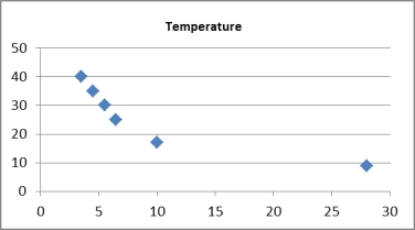 Scatterplot of Daily hot coffee sales revenue vs Temperature
 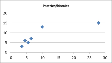 Scatterplot of Daily hot coffee sales revenue Pastries/biscuits
 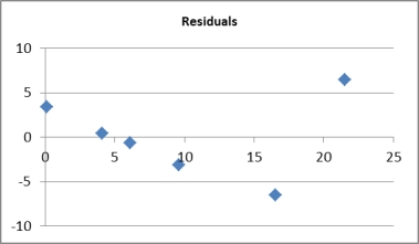 Residual scatterplot of Daily hot coffee sales revenue vs fitted values
(Essay)
4.7/5 (34)
Pop-up coffee vendors have been popular in the city of Adelaide in 2013. A Pop-up coffee vendor is interested in knowing how temperature (in degrees Celsius) and number of different pastries and biscuits offered to customers, impacts daily hot coffee sales revenue (in $00's).
A random sample of 6 days was taken, with the daily hot coffee sales revenue and the corresponding temperature and number of different pastries and biscuits offered on that day, noted.
Excel output for a multiple linear regression is given below: Coffee sales revenue Temperature Pastries/biscuits 6.5 25 7 10 17 13 5.5 30 5 4.5 35 6 3.5 40 3 28 9 15 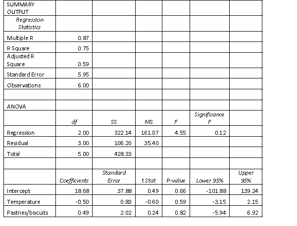 a. Write down the multiple regression model.
b. Interpret the coefficient of Temperature.
c. Interpret the coefficient of Pastries/biscuits.
a. Write down the multiple regression model.
b. Interpret the coefficient of Temperature.
c. Interpret the coefficient of Pastries/biscuits.
(Essay)
4.8/5 (35)
If multicollinearity exists among the independent variables included in a multiple regression model, then:
(Multiple Choice)
4.8/5 (25)
In a multiple regression model, the mean of the probability distribution of the error variable is assumed to be:
(Multiple Choice)
5.0/5 (30)
An economist wanted to develop a multiple regression model to enable him to predict the annual family expenditure on clothes. After some consideration, he developed the multiple regression model: .
Where:
y = annual family clothes expenditure (in $1000s) = annual household income (in $1000s) = number of family members = number of children under 10 years of age
The computer output is shown below.
THE REGRESSION EQUATION IS
Predictor Coef StDev Constant 1.74 0.630 2.762 0.091 0.025 3.640 0.93 0.290 3.207 0.26 0.180 1.444
ANALYSIS OF VARIANCE
Source of Variation df SS MS F Regression 3 288 96 22.647 Error 46 195 4.239 Total 49 483
Test at the 10% significance level to determine whether annual household income and annual family clothes expenditure are linearly related.
(Essay)
4.9/5 (39)
A multiple regression model has the form ŷ = b0 + b1x1 + b2x2. Which of the following best describes b2?
(Multiple Choice)
4.7/5 (40)
In order to test the significance of a multiple regression model involving 4 independent variables and 30 observations, the number of degrees of freedom for the numerator and denominator for the critical value of F are 4 and 26, respectively.
(True/False)
4.9/5 (40)
Multiple linear regression is used to estimate the linear relationship between one dependent variable and more than one independent variables.
(True/False)
4.9/5 (47)
When the independent variables are correlated with one another in a multiple regression analysis, this condition is called:
(Multiple Choice)
4.9/5 (31)
An actuary wanted to develop a model to predict how long individuals will live. After consulting a number of physicians, she collected the age at death (y), the average number of hours of exercise per week ( ), the cholesterol level ( ), and the number of points by which the individual's blood pressure exceeded the recommended value ( ). A random sample of 40 individuals was selected. The computer output of the multiple regression model is shown below:
THE REGRESSION EQUATION IS Predictor Coef StDev T Constant 55.8 11.8 4.729 1.79 0.44 4.068 -0.021 0.011 -1.909 -0.016 0.014 -1.143 S = 9.47 R-Sq = 22.5%. ANALYSIS OF VARIANCE Source of Variation df SS MS F Regression 3 936 312 3.477 Error 36 3230 89.722 Total 39 4166 Is there enough evidence at the 1% significance level to infer that the average number of hours of exercise per week and the age at death are linearly related?
(Essay)
4.8/5 (30)
The computer output for the multiple regression model is shown below. However, because of a printer malfunction some of the results are not shown. These are indicated by the boldface letters a to i. Fill in the missing results (up to three decimal places). Predictor Coef StDev Constant a 0.120 3.18 0.068 b 3.38 0.024 0.010 c S = d R-Sq = e. ANALYSIS OF VARIANCE Source of Variation df SS MS F Regression 2 7.382 g i Error 22 f h Total 24 7.530
(Essay)
4.9/5 (44)
An estimated multiple regression model has the form ŷ = 100 − 2x1 + 9x2. As x1 increases by 1 unit while holding x2 constant, which of the following best describes the change in y?
(Multiple Choice)
4.8/5 (40)
A statistician wanted to determine whether the demographic variables of age, education and income influence the number of hours of television watched per week. A random sample of 25 adults was selected to estimate the multiple regression model .
Where:
y = number of hours of television watched last week. = age. = number of years of education. = income (in $1000s).
The computer output is shown below.
THE REGRESSION EQUATION IS Predictor Coef StDev Constant 22.3 10.7 2.084 0.41 0.19 2.158 -0.29 0.13 -2.231 -0.12 0.03 -4.00 S = 4.51 R-Sq = 34.8%. ANALYSIS OF VARIANCE Source of Variation df SS MS F Regression 3 227 75.667 3.730 Error 21 426 20.286 Total 24 653 Is there sufficient evidence at the 1% significance level to indicate that hours of television watched and age are linearly related?
(Essay)
4.8/5 (40)
A multiple regression model has the form ŷ = 24 - 0.001x1 + 3x2.
As x1 increases by 1 unit, holding constant, the value of y is estimated to decrease by 0.001units, on average.
(True/False)
4.9/5 (38)
Which of the following measures can be used to assess a multiple regression model's fit?
(Multiple Choice)
4.8/5 (33)
In multiple regression, and because of a commonly occurring problem called multicollinearity, the
t-tests of the individual coefficients may indicate that some independent variables are not linearly related to the dependent variable, when in fact they are.
(True/False)
4.8/5 (39)
Which of the following best describes the range of the coefficient of multiple determination?
(Multiple Choice)
4.8/5 (32)
Filters
- Essay(0)
- Multiple Choice(0)
- Short Answer(0)
- True False(0)
- Matching(0)