Exam 19: Multiple Regression

A multiple regression analysis that includes 25 data points and 4 independent variables produces SST = 400 and SSR = 300. The multiple standard error of estimate will be 5.

An economist wanted to develop a multiple regression model to enable him to predict the annual family expenditure on clothes. After some consideration, he developed the multiple regression model: $y = \beta _ { 0 } + \beta _ { 1 } x _ { 1 } + \beta _ { 2 } x _ { 2 } + \beta _ { 3 } x _ { 3 } + \varepsilon$ . Where: y = annual family clothes expenditure (in $1000s) $x _ { 1 }$ = annual household income (in $1000s) $x _ { 2 }$ = number of family members $X _ { 3 }$ = number of children under 10 years of age The computer output is shown below. THE REGRESSION EQUATION IS $y=1.74+0.091 x_{1}+0.93 x_{2}+0.26 x_{3}$ Predictor Coef StDev T Constant 1.74 0.630 2.762 0.091 0.025 3.640 0.93 0.290 3.207 0.26 0.180 1.444 $\mathrm { S } = 2.06 \quad \mathrm { R } - \mathrm { Sq } = 59.6 \%$ ANALYSIS OF VARIANCE Source of Variation Regression 3 288 96 22.647 Error 46 195 4.239 Total 49 483 Test at the 1% significance level to determine whether the number of family members and annual family clothes expenditure are linearly related.

A statistics professor investigated some of the factors that affect an individual student's final grade in his or her course. He proposed the multiple regression model: $y = \beta _ { 0 } + \beta _ { 1 } x _ { 1 } + \beta _ { 2 } x _ { 2 } + \beta _ { 3 } x _ { 3 } + \varepsilon$ . Where: y = final mark (out of 100). $x _ { 1 }$ = number of lectures skipped. $x _ { 2 }$ = number of late assignments. $X _ { 3 }$ = mid-term test mark (out of 100). The professor recorded the data for 50 randomly selected students. The computer output is shown below. THE REGRESSION EQUATION IS $= 41.6 - 3.18 x _ { 1 } - 1.17 x _ { 2 } + .63 x _ { 3 }$ Predictor Coef StDev T Constant 41.6 17.8 2.337 -3.18 1.66 -1.916 -1.17 1.13 -1.035 0.63 0.13 4.846 $\mathrm { S } = 13.74 \quad \mathrm { R } - \mathrm { Sq } = 30.0 \%$ ANALYSIS OF VARIANCE Source of Variation df Regression 3 3716 1238.667 6.558 Error 46 8688 188.870 Total 49 12404 Do these data provide enough evidence to conclude at the 5% significance level that the model is useful in predicting the final mark?

An economist wanted to develop a multiple regression model to enable him to predict the annual family expenditure on clothes. After some consideration, he developed the multiple regression model: $y = \beta _ { 0 } + \beta _ { 1 } x _ { 1 } + \beta _ { 2 } x _ { 2 } + \beta _ { 3 } x _ { 3 } + \varepsilon$ . Where: y = annual family clothes expenditure (in $1000s) $x _ { 1 }$ = annual household income (in $1000s) $x _ { 2 }$ = number of family members $X _ { 3 }$ = number of children under 10 years of age The computer output is shown below. THE REGRESSION EQUATION IS $y =$ $1.74 + 0.091 x _ { 1 } + 0.93 x _ { 2 } + 0.26 x _ { 3 }$ Predictor Coef StDev Constant 1.74 0.630 2.762 0.091 0.025 3.640 0.93 0.290 3.207 0.26 0.180 1.444 S = 2.06 R-Sq = 59.6%. ANALYSIS OF VARIANCE Source of Variation df SS MS F Regression 3 288 96 22.647 Error 46 195 4.239 Total 49 483 Test the overall model's validity at the 5% significance level.

Consider the following statistics of a multiple regression model: n = 30 k = 4 SS_y = 1500 SSE = 260. a. Determine the standard error of estimate. b. Determine the multiple coefficient of determination. c. Determine the F-statistic.

In a regression model involving 60 observations, the following estimated regression model was obtained: $= 51.4 + 0.70 x _ { 1 } + 0.679 x _ { 2 } - 0.378 x _ { 3 }$ For this model, total variation in y = SSY = 119,724 and SSR = 29,029.72. The value of MSE is:

For the estimated multiple regression model = 30 -4x₁ + 5x₂ +3 x₃, a one unit increase in x₃, holding x₁ and x₂ constant, will result in which of the following changes in y?

In testing the validity of a multiple regression model in which there are four independent variables, the null hypothesis is:

An actuary wanted to develop a model to predict how long individuals will live. After consulting a number of physicians, she collected the age at death (y), the average number of hours of exercise per week ( $x _ { 1 }$ ), the cholesterol level ( $x _ { 2 }$ ), and the number of points by which the individual's blood pressure exceeded the recommended value ( $X _ { 3 }$ ). A random sample of 40 individuals was selected. The computer output of the multiple regression model is shown below: THE REGRESSION EQUATION IS $y =$ $55.8 + 1.79 x _ { 1 } - 0.021 x _ { 2 } - 0.016 x _ { 3 }$ Predictor Coef StDev T Constant 55.8 11.8 4.729 1.79 0.44 4.068 -0.021 0.011 -1.909 -0.016 0.014 -1.143 S = 9.47 R-Sq = 22.5%. ANALYSIS OF VARIANCE Source of Variation df SS MS F Regression 3 936 312 3.477 Error 36 3230 89.722 Total 39 4166 What is the coefficient of determination? What does this statistic tell you?

In multiple regression, the problem of multicollinearity affects the t-tests of the individual coefficients as well as the F-test in the analysis of variance for regression, since the F-test combines these t-tests into a single test.

An economist wanted to develop a multiple regression model to enable him to predict the annual family expenditure on clothes. After some consideration, he developed the multiple regression model: $y = \beta _ { 0 } + \beta _ { 1 } x _ { 1 } + \beta _ { 2 } x _ { 2 } + \beta _ { 3 } x _ { 3 } + \varepsilon$ . Where: y = annual family clothes expenditure (in $1000s) $x _ { 1 }$ = annual household income (in $1000s) $x _ { 2 }$ = number of family members $X _ { 3 }$ = number of children under 10 years of age The computer output is shown below. THE REGRESSION EQUATION IS $y = 1.74 + 0.091 x _ { 1 } + 0.93 x _ { 2 } + 0.26 x _ { 3 }$ Predictor Coef StDev T Constant 1.74 0.630 2.762 0.091 0.025 3.640 0.93 0.290 3.207 0.26 0.180 1.444 $\mathrm { S } = 2.06 \quad \mathrm { R } - \mathrm { Sq } = 59.6 \%$ ANALYSIS OF VARIANCE Source of Variation Regression 3 288 96 22.647 Error 46 195 4.239 Total 49 483 What is the coefficient of determination? What does this statistic tell you?

In reference to the equation $= 1.86 - 0.51 x _ { 1 } + 0.60 \quad x _ { 2 }$ , the value 0.60 is the change in $y$ per unit change in $x _ { 2 }$ , regardless of the value of $x _ { 1 }$ .

A statistics professor investigated some of the factors that affect an individual student's final grade in his or her course. He proposed the multiple regression model: $y = \beta _ { 0 } + \beta _ { 1 } x _ { 1 } + \beta _ { 2 } x _ { 2 } + \beta _ { 3 } x _ { 3 } + \varepsilon$ . Where: y = final mark (out of 100). $x _ { 1 }$ = number of lectures skipped. $x _ { 2 }$ = number of late assignments. $X _ { 3 }$ = mid-term test mark (out of 100). The professor recorded the data for 50 randomly selected students. The computer output is shown below. THE REGRESSION EQUATION IS = $41.6 - 3.18 x _ { 1 } - 1.17 x _ { 2 } + .63 x _ { 3 }$ Predictor Coef StDev T Constant 41.6 17.8 2.337 -3.18 1.66 -1.916 -1.17 1.13 -1.035 0.63 0.13 4.846 S = 13.74 R-Sq = 30.0%. ANALYSIS OF VARIANCE Source of Variation df SS MS F Regression 3 3716 1238.667 6.558 Error 46 8688 188.870 Total 49 12404 Do these data provide enough evidence at the 1% significance level to conclude that the final mark and the mid-term mark are positively linearly related?

A multiple regression analysis that includes 4 independent variables results in a sum of squares for regression of 1200 and a sum of squares for error of 800. The multiple coefficient of determination will be:

Test the hypotheses: $H _ { 0 } :$ There is no first-order autocorrelation $H _ { 1 } :$ There is first-order autocorrelation, given that the Durbin-Watson statistic d = 1.89, n = 28, k = 3 and $\alpha =$ 0.05.

Which of the following best describes a multiple linear regression model?

A multiple regression model has the form ŷ = b₀ + b₁x₁ + b₂x₂. The coefficient b₂ is interpreted as the change in $y$ per unit change in x₂.

In a multiple regression model, the standard deviation of the error variable $\varepsilon$ is assumed to be:

A multiple regression analysis that includes 20 data points and 4 independent variables results in total variation in y = SSY = 200 and SSR = 160. The multiple standard error of estimate will be:

Pop-up coffee vendors have been popular in the city of Adelaide in 2013. A vendor is interested in knowing how temperature (in degrees Celsius) and number of different pastries and biscuits offered to customers impacts daily hot coffee sales revenue (in $00's). A random sample of 6 days was taken, with the daily hot coffee sales revenue and the corresponding temperature and number of different pastries and biscuits offered on that day, noted. Excel output for a multiple linear regression is given below: Coffee sales revenue Temperature Pastries/biscuits 6.5 25 7 10 17 13 5.5 30 5 4.5 35 6 3.5 40 3 28 9 15 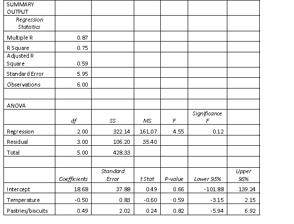Test the significance of the coefficient on Pasties/biscuits against a two tailed alternative. Use the 5% level of significance.