Exam 18: Simple Linear Regression and Correlation

If there is no linear relationship between two variables $x$ and $y$ , the coefficient of correclation will be zero.

An economist wanted to analyse the relationship between the speed of a car (x) in kilometres per hour (kmph) and its fuel consumption (y) in kilometres per litre (kmpl). In an experiment, a car was operated at several different speeds and for each speed the fuel consumption was measured. The data obtained are shown below. Speed (mph) 25 35 45 50 60 65 70 Fuel consumtion (mpg) 40 39 37 33 30 27 25 a. Find the least squares regression line. b. Calculate the standard error of estimate, and describe what this statistic tells you about the regression line. c. Do these data provide sufficient evidence at the 5% significance level to infer that a linear relationship exists between higher speeds and lower fuel consumption? d. Predict with 99% confidence the fuel consumption of a car traveling at 55 kmph.

In a simple linear regression model, if r² is 0.75, then 75% of the variation in the dependent variable y can be explained by the regression line, on the independent variable x.

At a recent music concert, a survey was conducted that asked a random sample of 20 people their age and how many concerts they have attended since the beginning of the year. The following data were collected. Age 62 57 40 49 67 54 43 65 54 41 Number of concerts 6 5 4 3 5 5 2 6 3 1 Age 44 48 55 60 59 63 69 40 38 52 Number of Concerts 3 2 4 5 4 5 4 2 1 3 SUMMARY OUTPUT DESCRIPTIVE STATISTICS Reqression Statiatics Multiple R 0.80203 R Square 0.64326 Adjusted R Square 0.62344 Standard Error 0.93965 Observations 20 Age Concerts Mean 53 Mean 3.65 Standard Error 2.1849 Standard Error 0.3424 Standard Deviation 9.7711 Standard Deviation 1.5313 Sample Variance 95.4737 Sample Variance 2.3447 Count 20 Count 20 $\text { SPEARMAN RANK CORRELATION COEFFICIENT }=0.8306$ ANOVA df SS MS F Significance F Regression 1 28.65711 28.65711 32.45653 2.1082-05 Residual 18 15.89289 0.88294 Total 19 44.55 Coefficients Standard Error t Stat P-value Lower 95\% Upper 95\% Intercept -3.01152 1.18802 -2.53491 0.02074 -5.50746 -0.5156 Age 0.12569 0.02206 5.69706 0.00002 0.07934 0.1720 a. Use the regression equation = -3.0115 + 0.1257x to determine the predicted values of y. b. Use the predicted values and the actual values of y to calculate the residuals. c. Plot the residuals against the predicted values . d. Does it appear that heteroscedasticity is a problem? Explain. e. Draw a histogram of the residuals. f. Does it appear that the errors are normally distributed? Explain. g. Use the residuals to compute the standardised residuals. h. Identify possible outliers.

Which of the following best describes the y-intercept in the simple linear regression model? \begin{array}{|l|l|}\hline\text { A. } & \text {The \mathrm{y} -intercept is the estimated average value of \( \mathrm{y} \) when \( \mathrm{x}=1 \). }\\\hline \text { B. } & \text { The \( \mathrm{y} \)-intercept is the estimated average value of \( \mathrm{x} \) when \( \mathrm{y}=0 \).} \\\hline \text { C. } &\text {The \( \mathrm{y} \)-intercept is the rate of change of \( \mathrm{y} \) with respect to changes in \( \mathrm{x} \). }\\\hline \text { D. } &\text { The \( \mathrm{y} \)-intercept is the estimated average value of \( \mathrm{y} \) when \( \mathrm{x}=0 \).}\\\hline\end{array}

The smallest value that the standard error of estimate $S _ { \varepsilon }$ can assume is: A. -1 B. 0. C. 1. D. -2.

The symbol for the population coefficient of correlation is: A r B \rho C D

The variance of the error variable, $\sigma _ { \varepsilon } ^ { 2 }$ , is required to be constant. When this requirement is violated, the condition is called heteroscedasticity.

If cov(X,Y) = -350, s_x² = 900 and s_y² = 225, then the coefficient of determination is: A. 0.8819 B. 0.7778. C. -0.0017 D. 0.0017.

Plot the residuals against the predicted values . Does the variance appear to be constant?

When the actual values y of a dependent variable and the corresponding predicted values are the same, the standard error of estimate, $S _ { \varepsilon }$ , will be -1.0.

At a recent music concert, a survey was conducted that asked a random sample of 20 people their age and how many concerts they have attended since the beginning of the year. The following data were collected. Age 62 57 40 49 67 54 43 65 54 41 Number of concerts 6 5 4 3 5 5 2 6 3 1 Age 44 48 55 60 59 63 69 40 38 52 Number of Concerts 3 2 4 5 4 5 4 2 1 3 SUMMARY OUTPUT DESCRIPTIVE STATISTICS Reqression Statiatics Multiple R 0.80203 R Square 0.64326 Adjusted R Square 0.62344 Standard Error 0.93965 Observations 20 Age Concerts Mean 53 Mean 3.65 Standard Error 2.1849 Standard Error 0.3424 Standard Deviation 9.7711 Standard Deviation 1.5313 Sample Variance 95.4737 Sample Variance 2.3447 Count 20 Count 20 $\text { SPEARMAN RANK CORRELATION COEFFICIENT }=0.8306$ ANOVA df SS MS F Significance F Regression 1 28.65711 28.65711 32.45653 2.1082-05 Residual 18 15.89289 0.88294 Total 19 44.55 Coefficients Standard Error t Stat P-value Lower 95\% Upper 95\% Intercept -3.01152 1.18802 -2.53491 0.02074 -5.50746 -0.5156 Age 0.12569 0.02206 5.69706 0.00002 0.07934 0.1720 a. Determine the standard error of estimate and describe what this statistic tells you about the model's fit. b. Interpret the coefficient of correlation. c. Interpret the coefficient of determination, and discuss what its value tells you about the two variables.

Given the data points (x,y) = (3,3), (4,4), (5,5), (6,6), (7,7), the least squares estimates of the y-intercept and slope are respectively: A. 0 and 1. B. -1 and 0. C. 5 and 5. D. 5 and 0.

The standard error of estimate, $S _ { \varepsilon}$ , is given by: A SSE (n-2) B /(n-2) C D SSE /

The standard error of estimate, $S _ { \varepsilon }$ , is a measure of: A. variation of y around the regression line B. variation of x around the regression line. C. variation of y around the mean . D. variation of x around the mean .

A financier whose specialty is investing in movie productions has observed that, in general, movies with 'big-name' stars seem to generate more revenue than those movies whose stars are less well known. To examine his belief, he records the gross revenue and the payment (in $ million) given to the two highest-paid performers in the movie for 10 recently released movies. Movie Cost of two highest- paid performers (\ ) Gross revenue (\ ) 1 5.3 48 2 7.2 65 3 1.3 18 4 1.8 20 5 3.5 31 6 2.6 26 7 8.0 73 8 2.4 23 9 4.5 39 10 6.7 58 Assume that the conditions for the tests conducted in the previous two questions are not met. Do the data allow us to infer at the 5% significance level that payment to the two highest-paid performers and gross revenue are linearly related?

A statistician investigating the relationship between the amount of precipitation (in inches) and the number of car accidents gathered data for 10 randomly selected days. The results are presented below. Day Precipitation Number of accidents 1 0.05 5 2 0.12 6 3 0.05 2 4 0.08 4 5 0.10 8 6 0.35 14 7 0.15 7 8 0.30 13 9 0.10 7 10 0.20 10 Find the least squares regression line.

Given that cov(x,y) = 8, $s _ { y } ^ { 2 }$ = 14, $S _ { x } ^ { 2 }$ = 10 and n = 6, the value of the sum of squares for error, SSE, is 38.

Which of the following best describes the relationship of the least squares regression line: Estimated y = 2 - x? A As x increases by 1 unit, y increases by 1 unit, estimated, on average. B As increases by 1 unit decreases by (2-) units, estimated, on average C As increases by 1 unit, y decreases by 1 unit, estimated, on average. D All of these choices are correct.

Pop-up coffee vendors have been popular in the city of Adelaide in 2013. A vendor is interested in knowing how temperature (in degrees Celsius) impacts daily hot coffee sales revenue (in $00's). A random sample of 6 days was taken, with the daily hot coffee sales revenue and the corresponding temperature of that day noted. Excel regression output given below. Coffee sales revenue Temperature 6.50 25 10.00 17 5.50 30 4.50 35 3.50 40 28.00 9 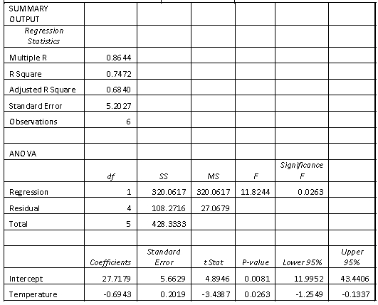(a) Estimate daily hot coffee sales revenue on a day of 38 degrees Celsius. (b) Is your prediction in part (a) reasonable?