Exam 18: Simple Linear Regression and Correlation

A statistician investigating the relationship between the amount of precipitation (in inches) and the number of car accidents gathered data for 10 randomly selected days. The results are presented below. Day Precipitation Number of accidents 1 0.05 5 2 0.12 6 3 0.05 2 4 0.08 4 5 0.10 8 6 0.35 14 7 0.15 7 8 0.30 13 9 0.10 7 10 0.20 10 Determine the coefficient of determination and discuss what its value tells you about the two variables.

At a recent music concert, a survey was conducted that asked a random sample of 20 people their age and how many concerts they have attended since the beginning of the year. The following data were collected. Age 62 57 40 49 67 54 43 65 54 41 Number of concerts 6 5 4 3 5 5 2 6 3 1 Age 44 48 55 60 59 63 69 40 38 52 Number of Concerts 3 2 4 5 4 5 4 2 1 3 SUMMARY OUTPUT DESCRIPTIVE STATISTICS Reqression Statiatics Multiple R 0.80203 R Square 0.64326 Adjusted R Square 0.62344 Standard Error 0.93965 Observations 20 Age Concerts Mean 53 Mean 3.65 Standard Error 2.1849 Standard Error 0.3424 Standard Deviation 9.7711 Standard Deviation 1.5313 Sample Variance 95.4737 Sample Variance 2.3447 Count 20 Count 20 $\text { SPEARMAN RANK CORRELATION COEFFICIENT }=0.8306$ ANOVA df SS MS F Significance F Regression 1 28.65711 28.65711 32.45653 2.1082-05 Residual 18 15.89289 0.88294 Total 19 44.55 Coefficients Standard Error t Stat P-value Lower 95\% Upper 95\% Intercept -3.01152 1.18802 -2.53491 0.02074 -5.50746 -0.5156 Age 0.12569 0.02206 5.69706 0.00002 0.07934 0.1720 a. Calculate the Pearson correlation coefficient. What sign does it have? Why? b. Conduct a test of the population coefficient of correlation to determine at the 5% significance level whether a linear relationship exists between age and number of concerts attended.

The manager of a fast food restaurant wants to determine how sales in a given week are related to the number of discount vouchers (#) printed in the local newspaper during the week. The number of vouchers and sales ($000s) from 10 randomly selected weeks is given below with Excel regression output. Number of vouchers Sales 4 12.8 7 15.4 5 13.9 3 11.2 19 18.7 10 17.9 8 16.8 6 15.9 3 11.5 5 13.9 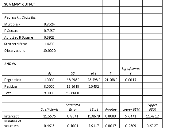Test the significance of the slope against a suitable alternative, at the 5% level of significance. Justify your choice of the direction in your alternative hypothesis.

The manager of a fast food restaurant wants to determine how sales in a given week are related to the number of discount vouchers (#) printed in the local newspaper during the week. The number of vouchers and sales ($000s) from 10 randomly selected weeks is given below with Excel regression output. Number of vouchers Sales 4 12.8 7 15.4 5 13.9 3 11.2 19 18.7 10 17.9 8 16.8 6 15.9 3 11.5 5 13.9 SUMMARY OUTPUT Regression Statistics Multiple R 0.8524 R Square 0.7267 Adjuted R Square 0.6925 Standard Error 1.4301 Observations 10.0000 ANOVA Sgnificance df SS MS F F Regression 1.0000 43.4982 43.4982 21.2682 0.0017 Residual 8.0000 16.3618 2.0452 Total 9.0000 59.8600 Coefficients Standard Error t Stat P-value Lower 95\% Upper 95\% Interoept 11.5676 0.8341 13.8679 0.0000 9.6441 13.4912 Number of voudhers 0.4618 0.1001 4.6117 0.0017 0.2309 0.6927 Interpret the coefficient of correlation.

The manager of a fast food restaurant wants to determine how sales in a given week are related to the number of discount vouchers (#) printed in the local newspaper during the week. The number of vouchers and sales ($000s) from 10 randomly selected weeks is given below with Excel regression output. Number of vouchers Sales 4 12.8 7 15.4 5 13.9 3 11.2 19 18.7 10 17.9 8 16.8 6 15.9 3 11.5 5 13.9 SUMMARY OUTPUT Regression Statistics Multiple R 0.8524 R Square 0.7267 Adjuted R Square 0.6925 Standard Error 1.4301 Observations 10.0000 ANOVA Sgnificance df SS MS F F Regression 1.0000 43.4982 43.4982 21.2682 0.0017 Residual 8.0000 16.3618 2.0452 Total 9.0000 59.8600 Coefficients Standard Error t Stat P-value Lower 95\% Upper 95\% Interoept 11.5676 0.8341 13.8679 0.0000 9.6441 13.4912 Number of voudhers 0.4618 0.1001 4.6117 0.0017 0.2309 0.6927 a. Write down the regression equation b. Interpret the slope.

An ardent fan of television game shows has observed that, in general, the more educated the contestant, the less money he or she wins. To test her belief, she gathers data about the last eight winners of her favourite game show. She records their winnings in dollars and their years of education. The results are as follows. Contestant Years of education Winnings 1 11 750 2 15 400 3 12 600 4 16 350 5 11 800 6 16 300 7 13 650 8 14 400 Predict with 95% confidence the winnings of a contestant who has 10 years of education.

In the first-order linear regression model, the population parameters of the y-intercept and the slope are: A. and B. and C. and D. and

A financier whose specialty is investing in movie productions has observed that, in general, movies with 'big-name' stars seem to generate more revenue than those movies whose stars are less well known. To examine his belief, he records the gross revenue and the payment (in $ million) given to the two highest-paid performers in the movie for 10 recently released movies. Movie Cost of two highest- paid performers (\ ) Gross revenue (\ ) 1 5.3 48 2 7.2 65 3 1.3 18 4 1.8 20 5 3.5 31 6 2.6 26 7 8.0 73 8 2.4 23 9 4.5 39 10 6.7 58 Conduct a test of the population slope to determine at the 5% significance level whether a linear relationship exists between payment to the two highest-paid performers and gross revenue.

A professor of economics wants to study the relationship between income y (in $1000s) and education x (in years). A random sample of eight individuals is taken and the results are shown below. Education 16 11 15 8 12 10 13 14 Income 58 40 55 35 43 41 52 49 Predict with 95% confidence the income of an individual with 10 years of education.

Pop-up coffee vendors have been popular in the city of Adelaide in 2013. A vendor is interested in knowing how temperature (in degrees Celsius) impacts daily hot coffee sales revenue (in $00's). A random sample of 6 days was taken, with the daily hot coffee sales revenue and the corresponding temperature of that day noted. Coffee sales revenue Temperature 6.50 25 10.00 17 5.50 30 4.50 35 3.50 40 28.00 9 Calculate and interpret a 95% confidence interval for the population slope.

The quality of oil is measured in API gravity degrees - the higher the degrees API, the higher the quality. The table shown below is produced by an expert in the field, who believes that there is a relationship between quality and price per barrel. Oil degrees API Frice per barrel (in \ ) 27.0 12.02 28.5 12.04 30.8 12.32 31.3 12.27 31.9 12.49 34.5 12.70 34.0 12.80 34.7 13.00 37.0 13.00 41.0 13.17 41.0 13.19 38.8 13.22 39.3 13.27 A partial Minitab output follows. Descriptive Statistics Variable Mean StDev SE Mean Degrees 13 34.60 4.613 1.280 Frice 13 12.730 0.457 0.127 Covariances Degrees Price Degrees 21.281667 Price 2.026750 0.208833 Regression Analysis Fredictor Coef StDev Constant 9.4349 0.2867 32.91 0.000 Degrees 0.095235 0.008220 11.59 0.000 S = 0.1314 R-Sq = 92.46% R-Sq(adj) = 91.7% Analysis of Variance Source DF SS MS F P Regression 1 2.3162 2.3162 134.24 0.000 Residual Error 11 0.1898 0.0173 Total 12 2.5060 Conduct a test of the population slope to determine at the 5% significance level whether a linear relationship exists between the quality of oil and price per barrel.

A professor of economics wants to study the relationship between income y (in $1000s) and education x (in years). A random sample of eight individuals is taken and the results are shown below. Education 16 11 15 8 12 10 13 14 Income 58 40 55 35 43 41 52 49 Determine the standard error of estimate, and describe what this statistic tells you about the regression line.

The least squares method for determining the best fit minimises: A. total variation in the dependent variable. B. the sum of squares for error. C. the sum of squares for regression. D. All of these choices are correct.

The standard error of the estimate is the standard deviation of the error variable.

A professor of economics wants to study the relationship between income y (in $1000s) and education x (in years). A random sample of eight individuals is taken and the results are shown below. Education 16 11 15 8 12 10 13 14 Income 58 40 55 35 43 41 52 49 Compute the standardised residuals.

Which of the following best describes the coefficient of determination? \begin{array}{|l|l|}\hline\text { A. } & \text { The coefficient of determination describes the percentage of variation in the \mathrm{x} }\\&\text { variable explained by the linear regression model on the y variable.}\\\hline \text { B. } & \text { The coefficient of determination describes the direction of variation in the \( y \) variable} \\&\text { explained by the linear regression model on the \( \mathrm{x} \) variable. }\\\hline \text { C. } &\text {The coefficient of determination describes the percentage of variation in the v variable explained }\\&\text { by the linear regression model on the \( \mathrm{x} \) variable. }\\\hline \text { D. } &\text { The coefficient of determination describes the percentage of variation in the y variable unexplained}\\&\text { by the linear regression model on the \( \mathrm{x} \) variable.}\\\hline\end{array}

A television rating wants to determine whether married couples tend to agree about the quality of the television shows they watch. Ten couples are asked to rate a particular comedy series on a 7-point scale where 1 = terrible and 7 = excellent. The results are shown below. Husband's rating 3 6 6 5 4 5 7 4 5 5 Wife's rating 5 5 4 5 4 4 6 3 4 5 Do these data provide sufficient evidence at the 5% significance level to conclude that the husband's and the wife's ratings are positively related?

A direct relationship between an independent variable x and a dependent variably y means that the variables x and y increase or decrease together.

Given that SSE = 150 and SSR = 450, the proportion of the variation in y that is explained by the variation in x is 0.75.

In simple linear regression, most often we perform a two-tail test of the population slope $\beta _ { 1 }$ to determine whether there is sufficient evidence to infer that a linear relationship exists. Which of the following best describes the null and alternative hypotheses needed for a test of significance? A :=0 :0 B :0 :=0 C :=0 :0 D :=0 :0