Exam 10: Correlation and Regression

The results for several randomly selected students for test 1 and test 2 grades are given below. Test 1 59 63 65 69 58 77 76 69 70 64 Test 2 72 67 78 82 75 87 92 83 87 78 Is there sufficient evidence to suggest that there is a linear correlation between test 1 and test 2 grades? Construct a scatterplot, and find the value of the linear correlation coefficient r . Also, find the P -value or the critical value(s) of r using $\alpha = 0.05$

Given the linear correlation coefficient r and the sample size n, determine the critical values of r and use your finding to state whether or not the given r represents a significant linear correlation. Use a significance level of 0.05. R = 0.543, n = 25

Use the given data to find the equation of the regression line. Round the final values to three significant digits, if necessary. x 1 3 5 7 9 y 143 116 100 98 90

Find the explained variation for the paired data. The equation of the regression line for the paired data below is $\hat { y } = 6.18286 + 4.33937 x$ 9 7 2 3 4 22 17 43 35 16 21 23 102 81

When testing to determine if correlation is significant, we use the hypotheses $H _ { 0 }$ p=0 , $H _ { 1 } : \rho \neq 0$ What does the symbol $\rho$ represent? Explain the meaning of the null and alternative hypotheses.

The following table gives the US domestic oil production rates (excluding Alaska) from 1987 to 2002. A regression equation was fit to the data and the residual plot is shown below. Year Millions of Barrels per Day Year Millions of Barrels per Day 1987 6.39 1995 5.08 1988 6.12 1996 5.07 1989 5.74 1997 5.16 1990 5.58 1998 5.08 1991 5.62 1999 4.83 1992 5.46 2000 4.85 1993 5.26 2001 4.84 1994 5.10 2002 4.83 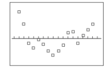Does the residual plot suggest that the regression equation is a bad model? why or why not?

For each of 200 randomly selected cities, Pete recorded the number of churches in the city (x)and the number of homicides in the past decade (y). He calculated the linear correlation coefficient and was surprised to find a strong positive linear correlation for the two variables. Does this suggest that building new churches causes an increase in the number of homicides? Why do you think that a strong positive linear correlation coefficient was obtained? Explain your answer with reference to the term lurking variable.

Suppose you will perform a test to determine whether there is sufficient evidence to support a claim of a linear correlation between two variables. Find the critical values of r given the number of pairs of data n and the significance level $\alpha$ n=14, $\alpha = 0.01$

Give an example of a pair of variables which you would expect to have a negative linear correlation coefficient and explain why.

A set of data consists of the number of years that applicants for foreign service jobs have studied German and the grades that they received on a proficiency test. The following regression equation is obtained: $\hat { y } = 31.6 + 10.9 x$ where x represents the number of years of study and y represents the grade on the test. Identify the predictor and response variables.

Use the given data to find the equation of the regression line. Round the final values to three significant digits, if necessary. Two different tests are designed to measure employee productivity and dexterity. Several employees are randomly selected and tested with these Results. Productivity (x) 23 25 28 21 21 25 26 30 34 36 Dexterity (y) 49 53 59 42 47 53 55 63 67 75

The table below lists weights (carats) and prices (dollars) for randomly selected diamonds. Is there sufficient evidence to suggest that there is a linear correlation between weights and prices? Construct a scatterplot, and find the value of the linear correlation coefficient r . Also find the P -value or the critical values of r using $\alpha = 0.05$ Weight 0.3 0.4 0.5 0.5 1.0 0.7 Price 510 1151 1343 1410 5669 2277

Construct a scatterplot for the given data. x 0.33 0.92 0.36 0.29 -0.09 0.97 0.39 0.3 y 0.5 0.49 0.08 0.27 -0.13 0.44 0.95 -0.09

The table lists the value y (in dollars) of $100 desposit (CD) at a bank after y years. Year 1 2 3 4 5 20 Value 103 106.09 109.27 112.55 115.93 180.61 Construct a scatterplot and identify the mathematical model that best fits the given data. Assume that the model is to be used only for the scope of the given data, and consider only linear, quadratic, logarithmic, exponential, and power models. Include the type of model and the equation for the model you find.

Find the unexplained variation for the paired data. The equation of the regression line for the paired data below is y=3x. 2 4 5 6 7 11 13 20

Use computer software to find the multiple regression equation. Can the equation be used for prediction? A wildlife analyst gathered the data in the table to develop an equation to predict the weights of bears. He used WEIGHT as the dependent variable and CHEST, LENGTH, And SEX as the independent variables. For SEX, he used male=1 and female=2. WEIGHT CHEST LENGTH SEX 344 45.0 67.5 1 416 54.0 72.0 1 220 41.0 70.0 2 360 49.0 68.5 1 332 44.0 73.0 1 140 32.0 63.0 2 436 48.0 72.0 1 132 33.0 61.0 2 356 48.0 64.0 2 150 35.0 59.0 1 202 40.0 63.0 2 365 50.0 70.5 1

Find the indicated multiple regression equation. Below are performance and attitude ratings of employees. Performance 59 63 65 69 58 77 76 69 70 64 Attitude 72 67 78 82 75 87 92 83 87 78 Managers also rate the same employees according to adaptability, and below are the results that correspond to those given above. Adaptability : 50 52 54 60 46 67 66 59 62 55 Find the multiple regression equation that expresses performance in terms of attitude and adaptability.

Describe what scatterplots are and discuss the importance of creating scatterplots.

Use the given data to find the equation of the regression line. Round the final values to three significant digits, if necessary. x 6 8 20 28 36 y 2 4 13 20 30

Use computer software to find the multiple regression equation. Can the equation be used for prediction? An anti-smoking group used data in the table to relate the carbon monoxide( CO) of various brands of cigarettes to their tar and nicotine (NIC)content. TAR NIC 15 1.2 16 15 1.2 16 17 1.0 16 6 0.8 9 1 0.1 1 8 0.8 8 10 0.8 10 17 1.0 16 15 1.2 15 11 0.7 9 18 1.4 18 16 1.0 15 10 0.8 9 7 0.5 5 18 1.1 16