Exam 3: Review of Statistics

L Let $Y$ be a Bernoulli random variable with success probability $\operatorname { Pr } ( Y = 1 ) = p$ , and let $Y _ { 1 } , \ldots , Y _ { n }$ be i.i.d. draws from this distribution. Let $\hat { p }$ be the fraction of successes (1s) in this sample. Given the following statement $\operatorname { Pr } ( - 1.96 < z < 1.96 ) = 0.95$ and assuming that $\hat { p }$ being approximately distributed $N \left( p , \frac { p ( 1 - p ) } { n } \right)$ , derive the $95 \%$ confidence interval for $p$ by solving the above inequalities.

An estimator $\hat { \mu } _ { Y }$ of the population value $\mu _ { Y }$ is unbiased if

The power of the test is a. dependent on whether you calculate a $t$ or a $t ^ { 2 }$ statistic. b. one minus the probability of committing a type I error. c. a subjective view taken by the econometrician dependent on the situation. d. one minus the probability of committing a type II error.

When the sample size n is large, the 90% confidence interval for $\mu _ { Y }$ is

Your textbook defines the correlation coefficient as follows: $r = \frac { \frac { 1 } { n - 1 } \sum _ { i = 1 } ^ { n } \left( Y _ { i } - \bar { Y } \right) ^ { 2 } \left( X _ { i } - \bar { X } \right) ^ { 2 } } { \sqrt { \frac { 1 } { n - 1 } \sum _ { i = 1 } ^ { n } \left( Y _ { i } - \bar { Y } \right) ^ { 2 } } \sqrt { \frac { 1 } { n - 1 } \sum _ { i = 1 } ^ { n } \left( X _ { i } - \bar { X } \right) ^ { 2 } } }$ Another textbook gives an alternative formula: $r = \frac { n \sum _ { i = 1 } ^ { n } Y _ { i } X _ { i } - \left( \sum _ { i = 1 } ^ { n } Y _ { i } \right) \left( \sum _ { i = 1 } ^ { n } X _ { i } \right) } { \sqrt { n \sum _ { i = 1 } ^ { n } Y _ { i } ^ { 2 } - \left( \sum _ { i = 1 } ^ { n } Y _ { i } \right) ^ { 2 } } \sqrt { n \sum _ { i = 1 } ^ { n } X _ { i } ^ { 2 } - \left( \sum _ { i = 1 } ^ { n } X _ { i } \right) ^ { 2 } } }$ Prove that the two are the same. 22

Some policy advisors have argued that education should be subsidized in developing countries to reduce fertility rates.To investigate whether or not education and fertility are correlated, you collect data on population growth rates (Y)and education (X)for 86 countries.Given the sums below, compute the sample correlation: $\sum _ { i = 1 } ^ { n } Y _ { i } = 1.594 ; \sum _ { i = 1 } ^ { n } X _ { i } = 449.6 ; \sum _ { i = 1 } ^ { n } Y _ { i } X _ { i } = 6.4697 ; \sum _ { i = 1 } ^ { n } Y _ { i } ^ { 2 } = 0.03982 ; \sum _ { i = 1 } ^ { n } X _ { i } ^ { 2 } = 3,022.76$

When you perform hypothesis tests, you are faced with four possible outcomes described in the accompanying table. 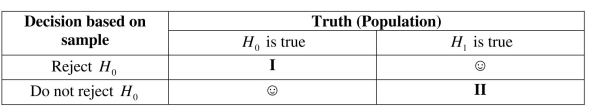“☺" indicates a correct decision, and I and II indicate that an error has been made. In probability terms, state the mistakes that have been made in situation I and II, and relate these to the Size of the test and the Power of the test (or transformations of these).

Among all unbiased estimators that are weighted averages of $Y _ { 1 } , \ldots , Y _ { n } , \bar { Y }$ is

A large p -value implies

Imagine that you had sampled 1,000,000 females and 1,000,000 males to test whether or not females have a higher IQ than males.IQs are normally distributed with a mean of 100 and a standard deviation of 16.You are excited to find that females have an average IQ of 101 in your sample, while males have an IQ of 99.Does this difference seem important? Do you really need to carry out a t-test for differences in means to determine whether or not this difference is statistically significant? What does this result tell you about testing hypotheses when sample sizes are very large?

Your textbook suggests using the first observation from a sample of n as an estimator of the population mean.It is shown that this estimator is unbiased but has a variance of σ2 , which makes it less efficient than the sample mean.Explain why this estimator is Y not consistent.You develop another estimator, which is the simple average of the first and last observation in your sample.Show that this estimator is also unbiased and show that it is more efficient than the estimator which only uses the first observation.Is this estimator consistent?

L Let $Y$ be a Bernoulli random variable with success probability $\operatorname { Pr } ( Y = 1 ) = p$ , and let $Y _ { 1 } , \ldots , Y _ { n }$ be i.i.d. draws from this distribution. Let $\hat { p }$ be the fraction of successes (1s) in this sample. In large samples, the distribution of $\hat { p }$ will be approximately normal, i.e., $\hat { p }$ is approximately distributed $N \left( p , \frac { p ( 1 - p ) } { n } \right)$ . Now let $X$ be the number of successes and $n$ the sample size. In a sample of 10 voters $( n = 10 )$ , if there are six who vote for candidate $\mathrm { A }$ , then $X = 6$ . Relate $X$ , the number of success, to $\hat { p }$ , the success proportion, or fraction of successes. Next, using your knowledge of linear transformations, derive the distribution of $X$ . 24

A manufacturer claims that a certain brand of VCR player has an average life expectancy of 5 years and 6 months with a standard deviation of 1 year and 6 months. Assume that the life expectancy is normally distributed. (a)Selecting one VCR player from this brand at random, calculate the probability of its life expectancy exceeding 7 years.

If the null hypothesis states $H _ { 0 } : E ( Y ) = \mu _ { Y , 0 }$ , then a two-sided alternative hypothesis is

The net weight of a bag of flour is guaranteed to be 5 pounds with a standard deviation of 0.05 pounds.You are concerned that the actual weight is less.To test for this, you sample 25 bags.Carefully state the null and alternative hypothesis in this situation. Determine a critical value such that the size of the test does not exceed 5%.Finding the average weight of the 25 bags to be 4.7 pounds, can you reject the null hypothesis? What is the power of the test here? Why is it so low?

When you are testing a hypothesis against a two-sided alternative, then the alternative is written as a. $E ( Y ) > \mu _ { Y , 0 }$ . b. $E ( Y ) = \mu _ { Y , 0 }$ . c. $\bar { Y } \neq \mu _ { Y , 0 }$ . d. $\quad E ( Y ) \neq \mu _ { Y , 0 }$ .

The critical value of a two-sided t-test computed from a large sample

Assume that under the null hypothesis, $\bar { Y }$ has an expected value of 500 and a standard deviation of 20. Under the alternative hypothesis, the expected value is 550 . Sketch the probability density function for the null and the alternative hypothesis in the same figure. Pick a critical value such that the $p$ -value is approximately 5\%. Mark the areas, which show the size and the power of the test. What happens to the power of the test if the alternative hypothesis moves closer to the null hypothesis, i.e., $\mu _ { Y } = 540,530,520$ , etc.? 25

The size of the test

During the last few days before a presidential election, there is a frenzy of voting intention surveys.On a given day, quite often there are conflicting results from three major polls. (a) Think of each of these polls as reporting the fraction of successes (1s) of a Bernoulli random variable $Y$ , where the probability of success is $\operatorname { Pr } ( Y = 1 ) = p$ . Let $\hat { p }$ be the fraction of successes in the sample and assume that this estimator is normally distributed with a mean of $p$ and a variance of $\frac { p ( 1 - p ) } { n }$ . Why are the results for all polls different, even though they are taken on the same day?