Exam 14: Introduction to Multiple Regression

SCENARIO 14-4 A real estate builder wishes to determine how house size (House)is influenced by family income (Income)and family size (Size).House size is measured in hundreds of square feet and income is measured in thousands of dollars.The builder randomly selected 50 families and ran the multiple regression.Partial Microsoft Excel output is provided below: 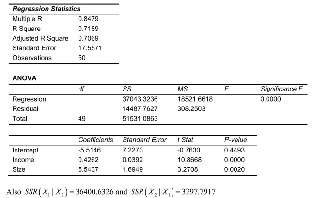-Referring to Scenario 14-4, what is the predicted house size (in hundreds of square feet)for an individual earning an annual income of $40,000 and having a family size of 4?

SCENARIO 14-7 The department head of the accounting department wanted to see if she could predict the GPA of students using the number of course units and total SAT scores of each.She takes a sample of students and generates the following Microsoft Excel output: 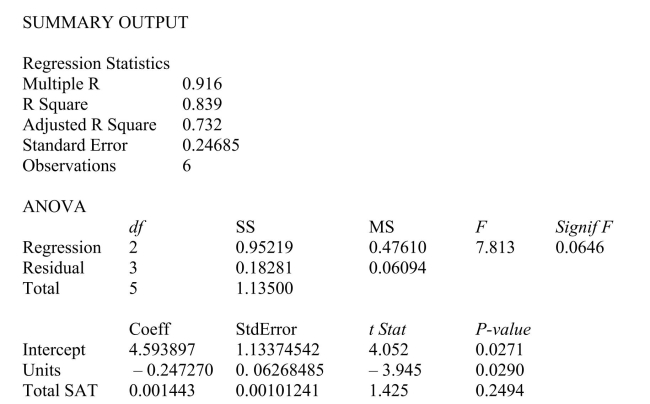-Referring to Scenario 14-7, the department head wants to use a t test to test for the significance of the coefficient of The value of the test statistic is ________.

SCENARIO 14-8 A financial analyst wanted to examine the relationship between salary (in $1,000)and 2 variables: age = Age)and experience in the field = Exper).He took a sample of 20 employees and obtained the following Microsoft Excel output: 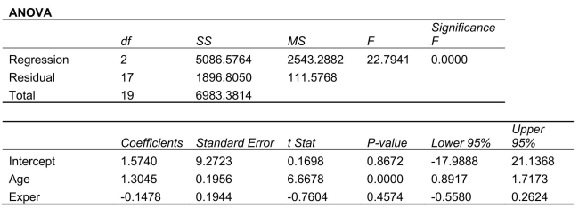Also, the sum of squares due to the regression for the model that includes only Age is 5022.0654 while the sum of squares due to the regression for the model that includes only Exper is 125.9848. -Referring to Scenario 14-8, the predicted salary (in $1,000)for a 35-year-old person with 10 years of experience is ________.

SCENARIO 14-15 The superintendent of a school district wanted to predict the percentage of students passing a sixth-grade proficiency test.She obtained the data on percentage of students passing the proficiency test (% Passing), mean teacher salary in thousands of dollars (Salaries), and instructional spending per pupil in thousands of dollars (Spending)of 47 schools in the state. 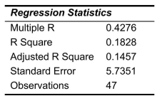Following is the multiple regression output with Y = % Passing as the dependent variable, = Salaries and Spending: -Referring to Scenario 14-15, you can conclude definitively that instructional spending per pupil individually has no impact on the mean percentage of students passing the proficiency test, considering the effect of mean teacher salary, at a 1% level of significance based solely on but not actually computing the 99% the confidence interval estimate for

SCENARIO 14-8 A financial analyst wanted to examine the relationship between salary (in $1,000)and 2 variables: age = Age)and experience in the field = Exper).He took a sample of 20 employees and obtained the following Microsoft Excel output: Also, the sum of squares due to the regression for the model that includes only Age is 5022.0654 while the sum of squares due to the regression for the model that includes only Exper is 125.9848. -Referring to Scenario 14-8, the coefficient of partial determination is ____.

SCENARIO 14-15 The superintendent of a school district wanted to predict the percentage of students passing a sixth-grade proficiency test.She obtained the data on percentage of students passing the proficiency test (% Passing), mean teacher salary in thousands of dollars (Salaries), and instructional spending per pupil in thousands of dollars (Spending)of 47 schools in the state. Following is the multiple regression output with Y = % Passing as the dependent variable, = Salaries and Spending: -Referring to Scenario 14-15, what is the standard error of estimate?

SCENARIO 14-8 A financial analyst wanted to examine the relationship between salary (in $1,000)and 2 variables: age = Age)and experience in the field = Exper).He took a sample of 20 employees and obtained the following Microsoft Excel output: Also, the sum of squares due to the regression for the model that includes only Age is 5022.0654 while the sum of squares due to the regression for the model that includes only Exper is 125.9848. -Referring to Scenario 14-8, the partial F test for : Variable does not significantly improve the model after variable has been included : Variable significantly improves the model after variable has been included has ____ and ____ degrees of freedom.

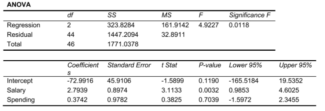
SCENARIO 14-17 Given below are results from the regression analysis where the dependent variable is the number of weeks a worker is unemployed due to a layoff (Unemploy)and the independent variables are the age of the worker (Age)and a dummy variable for management position (Manager: 1 = yes, 0 = no). The results of the regression analysis are given below: 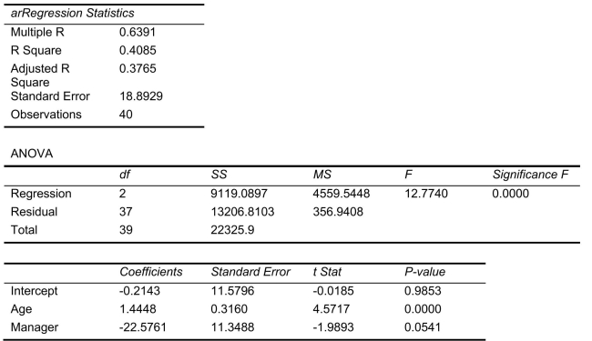-Referring to Scenario 14-17, the null hypothesis should be rejected at a 10% level of significance when testing whether age has any effect on the number of weeks a worker is unemployed due to a layoff while holding constant the effect of the other independent variable.

SCENARIO 14-4 A real estate builder wishes to determine how house size (House)is influenced by family income (Income)and family size (Size).House size is measured in hundreds of square feet and income is measured in thousands of dollars.The builder randomly selected 50 families and ran the multiple regression.Partial Microsoft Excel output is provided below: -Referring to Scenario 14-4, what annual income (in thousands of dollars)would an individual with a family size of 9 need to attain a predicted 5,000 square foot home (House = 50)?

SCENARIO 14-4 A real estate builder wishes to determine how house size (House)is influenced by family income (Income)and family size (Size).House size is measured in hundreds of square feet and income is measured in thousands of dollars.The builder randomly selected 50 families and ran the multiple regression.Partial Microsoft Excel output is provided below: -Referring to Scenario 14-4, suppose the builder wants to test whether the coefficient on Size is significantly different from 0.What is the value of the relevant t-statistic?

SCENARIO 14-15 The superintendent of a school district wanted to predict the percentage of students passing a sixth-grade proficiency test.She obtained the data on percentage of students passing the proficiency test (% Passing), mean teacher salary in thousands of dollars (Salaries), and instructional spending per pupil in thousands of dollars (Spending)of 47 schools in the state. Following is the multiple regression output with Y = % Passing as the dependent variable, = Salaries and Spending: -Referring to Scenario 14-15, the alternative hypothesis : At least one of for j = 1, 2 implies that percentage of students passing the proficiency test is related to both of the explanatory variables.

SCENARIO 14-17 Given below are results from the regression analysis where the dependent variable is the number of weeks a worker is unemployed due to a layoff (Unemploy)and the independent variables are the age of the worker (Age)and a dummy variable for management position (Manager: 1 = yes, 0 = no). The results of the regression analysis are given below: -Referring to Scenario 14-17, which of the following is the correct alternative hypothesis to test whether age has any effect on the number of weeks a worker is unemployed due to a layoff while holding constant the effect of the other independent variable?

SCENARIO 14-10 You worked as an intern at We Always Win Car Insurance Company last summer.You notice that individual car insurance premiums depend very much on the age of the individual and the number of traffic tickets received by the individual.You performed a regression analysis in EXCEL and obtained the following partial information: -Referring to Scenario 14-10, to test the significance of the multiple regression model, the value of the test statistic is ______.

SCENARIO 14-6 One of the most common questions of prospective house buyers pertains to the cost of heating in dollars (Y).To provide its customers with information on that matter, a large real estate firm used the following 2 variables to predict heating costs: the daily minimum outside temperature in degrees of Fahrenheit and the amount of insulation in inches Given below is EXCEL output of the regression model. 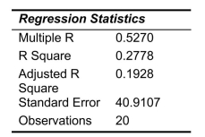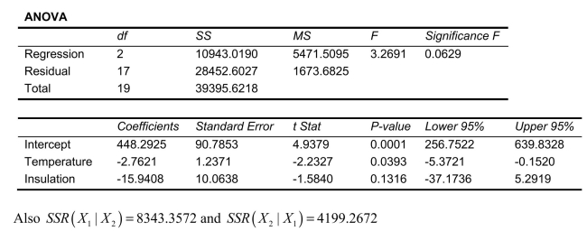-Referring to Scenario 14-6, the estimated value of the regression parameter in means that

SCENARIO 14-4 A real estate builder wishes to determine how house size (House)is influenced by family income (Income)and family size (Size).House size is measured in hundreds of square feet and income is measured in thousands of dollars.The builder randomly selected 50 families and ran the multiple regression.Partial Microsoft Excel output is provided below: -Referring to Scenario 14-4, when the builder used a simple linear regression model with house size (House)as the dependent variable and family size (Size)as the independent variable, he obtained an r2 value of 1.25%.What additional percentage of the total variation in house size has been explained by including income in the multiple regression?

SCENARIO 14-8 A financial analyst wanted to examine the relationship between salary (in $1,000)and 2 variables: age = Age)and experience in the field = Exper).He took a sample of 20 employees and obtained the following Microsoft Excel output: Also, the sum of squares due to the regression for the model that includes only Age is 5022.0654 while the sum of squares due to the regression for the model that includes only Exper is 125.9848. -Referring to Scenario 14-8, ____% of the variation in salary can be explained by the variation in age while holding experience constant.

In a particular model, the sum of the squared residuals was 847.If the model had 5 independent variables, and the data set contained 40 points, the value of the standard error of the estimate is 24.912.

SCENARIO 14-19 The marketing manager for a nationally franchised lawn service company would like to study the characteristics that differentiate home owners who do and do not have a lawn service.A random sample of 30 home owners located in a suburban area near a large city was selected; 11 did not have a lawn service (code 0)and 19 had a lawn service (code 1).Additional information available concerning these 30 home owners includes family income (Income, in thousands of dollars)and lawn size (Lawn Size, in thousands of square feet). The PHStat output is given below: 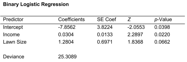-Referring to Scenario 14-19, there is not enough evidence to conclude that the model is not a good-fitting model at a 0.05 level of significance.

SCENARIO 14-15 The superintendent of a school district wanted to predict the percentage of students passing a sixth-grade proficiency test.She obtained the data on percentage of students passing the proficiency test (% Passing), mean teacher salary in thousands of dollars (Salaries), and instructional spending per pupil in thousands of dollars (Spending)of 47 schools in the state. Following is the multiple regression output with Y = % Passing as the dependent variable, = Salaries and Spending: -Referring to Scenario 14-15, the null hypothesis 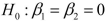implies that percentage of students passing the proficiency test is not affected by one of the explanatory variables.

SCENARIO 14-15 The superintendent of a school district wanted to predict the percentage of students passing a sixth-grade proficiency test.She obtained the data on percentage of students passing the proficiency test (% Passing), mean teacher salary in thousands of dollars (Salaries), and instructional spending per pupil in thousands of dollars (Spending)of 47 schools in the state. Following is the multiple regression output with Y = % Passing as the dependent variable, = Salaries and Spending: -Referring to Scenario 14-15, you can conclude definitively that instructional spending per pupil individually has no impact on the mean percentage of students passing the proficiency test, considering the effect of mean teacher salary, at a 10% level of significance based solely on but not actually computing the 90% confidence interval estimate for