Exam 15: Multiple Regression Model Building

SCENARIO 15-6 Given below are results from the regression analysis on 40 observations where the dependent variable is the number of weeks a worker is unemployed due to a layoff (Y)and the independent variables are the age of the worker ( ), the number of years of education received ( ), the number of years at the previous job ( ), a dummy variable for marital status ( 1 = married, 0 = otherwise), a dummy variable for head of household ( 1 = yes, 0 = no)and a dummy variable for management position ( 1 = yes, 0 = no). The coefficient of multiple determination ( )for the regression model using each of the 6 variables as the dependent variable and all other X variables as independent variables are, respectively, 0.2628, 0.1240, 0.2404, 0.3510, 0.3342 and 0.0993. The partial results from best-subset regression are given below: 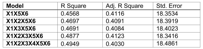-Referring to Scenario 15-6, what is the value of the Mallow's statistic for the model that includes all the six independent variables?

A real estate builder wishes to determine how house size (House)is influenced by family income (Income), family size (Size), and education of the head of household (School). House size is measured in hundreds of square feet, income is measured in thousands of dollars, and education is in years.The builder randomly selected 50 families and constructed the multiple regression model.The business literature involving human capital shows that education influences an individual's annual income.Combined, these may influence family size.With this in mind, what should the real estate builder be particularly concerned with when analyzing the multiple regression model?

SCENARIO 15-6 Given below are results from the regression analysis on 40 observations where the dependent variable is the number of weeks a worker is unemployed due to a layoff (Y)and the independent variables are the age of the worker ( ), the number of years of education received ( ), the number of years at the previous job ( ), a dummy variable for marital status ( 1 = married, 0 = otherwise), a dummy variable for head of household ( 1 = yes, 0 = no)and a dummy variable for management position ( 1 = yes, 0 = no). The coefficient of multiple determination ( )for the regression model using each of the 6 variables as the dependent variable and all other X variables as independent variables are, respectively, 0.2628, 0.1240, 0.2404, 0.3510, 0.3342 and 0.0993. The partial results from best-subset regression are given below: -Referring to Scenario 15-6, the variable x₁ should be dropped to remove collinearity?

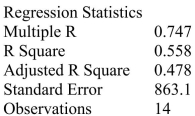
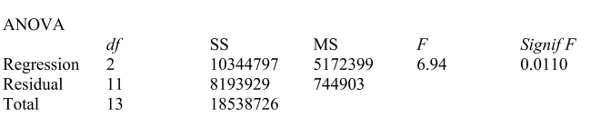
SCENARIO 15-3 A chemist employed by a pharmaceutical firm has developed a muscle relaxant.She took a sample of 14 people suffering from extreme muscle constriction.She gave each a vial containing a dose (X)of the drug and recorded the time to relief (Y)measured in seconds for each.She fit a curvilinear model to this data.The results obtained by Microsoft Excel follow SUMMARY OUTPUT 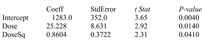-Referring to Scenario 15-3, the prediction of time to relief for a person receiving a dose of 10 units of the drug is ________.

Which of the following regression procedures are needed when the dependent variable is categorical?

SCENARIO 15-6 Given below are results from the regression analysis on 40 observations where the dependent variable is the number of weeks a worker is unemployed due to a layoff (Y)and the independent variables are the age of the worker ( ), the number of years of education received ( ), the number of years at the previous job ( ), a dummy variable for marital status ( 1 = married, 0 = otherwise), a dummy variable for head of household ( 1 = yes, 0 = no)and a dummy variable for management position ( 1 = yes, 0 = no). The coefficient of multiple determination ( )for the regression model using each of the 6 variables as the dependent variable and all other X variables as independent variables are, respectively, 0.2628, 0.1240, 0.2404, 0.3510, 0.3342 and 0.0993. The partial results from best-subset regression are given below: -Referring to Scenario 15-6, the model that includes should be among the appropriate models using the Mallow's statistic.

SCENARIO 15-6 Given below are results from the regression analysis on 40 observations where the dependent variable is the number of weeks a worker is unemployed due to a layoff (Y)and the independent variables are the age of the worker ( ), the number of years of education received ( ), the number of years at the previous job ( ), a dummy variable for marital status ( 1 = married, 0 = otherwise), a dummy variable for head of household ( 1 = yes, 0 = no)and a dummy variable for management position ( 1 = yes, 0 = no). The coefficient of multiple determination ( )for the regression model using each of the 6 variables as the dependent variable and all other X variables as independent variables are, respectively, 0.2628, 0.1240, 0.2404, 0.3510, 0.3342 and 0.0993. The partial results from best-subset regression are given below: -Referring to Scenario 15-6, what is the value of the variance inflationary factor of Head?

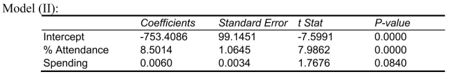
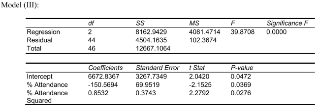
SCENARIO 15-4 The superintendent of a school district wanted to predict the percentage of students passing a sixth-grade proficiency test.She obtained the data on percentage of students passing the proficiency test (% Passing), daily mean of the percentage of students attending class (% Attendance), mean teacher salary in dollars (Salaries), and instructional spending per pupil in dollars (Spending)of 47 schools in the state. Let Y = % Passing as the dependent variable, Attendance, Salaries and Spending. The coefficient of multiple determination ( )of each of the 3 predictors with all the other remaining predictors are, respectively, 0.0338, 0.4669, and 0.4743. 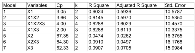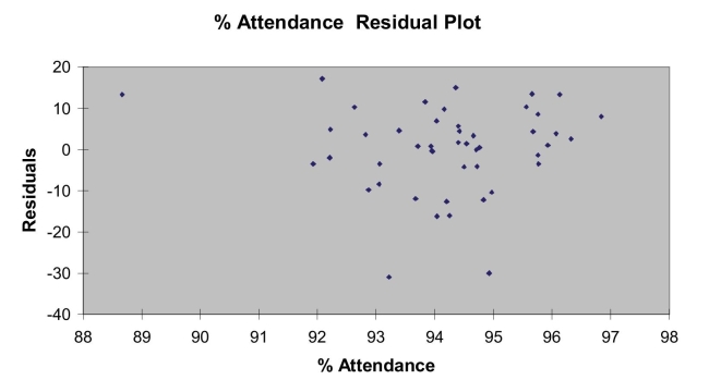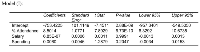The output from the best-subset regressions is given below: Following is the residual plot for % Attendance: Following is the output of several multiple regression models: -Referring to Scenario 15-4, the residual plot suggests that a nonlinear model on % attendance may be a better model.

In data mining where huge data sets are being explored to discover relationships among a large number of variables, the best-subsets approach is more practical than the stepwise regression approach.

Collinearity is present when there is a high degree of correlation between independent variables.

In multiple regression, the __________ procedure permits variables to enter and leave the model at different stages of its development.

A regression diagnostic tool used to study the possible effects of collinearity is ______.

SCENARIO 15-4 The superintendent of a school district wanted to predict the percentage of students passing a sixth-grade proficiency test.She obtained the data on percentage of students passing the proficiency test (% Passing), daily mean of the percentage of students attending class (% Attendance), mean teacher salary in dollars (Salaries), and instructional spending per pupil in dollars (Spending)of 47 schools in the state. Let Y = % Passing as the dependent variable, Attendance, Salaries and Spending. The coefficient of multiple determination ( )of each of the 3 predictors with all the other remaining predictors are, respectively, 0.0338, 0.4669, and 0.4743. The output from the best-subset regressions is given below: Following is the residual plot for % Attendance: Following is the output of several multiple regression models: -Referring to Scenario 15-4, The superintendent wants to know the quadratic effect of average percentage of students attending class on the percentage of students passing the proficiency test.What is the value of the test statistic?

SCENARIO 15-1 A certain type of rare gem serves as a status symbol for many of its owners.In theory, for low prices, the demand increases, and it decreases as the price of the gem increases.However, experts hypothesize that when the gem is valued at very high prices, the demand increases with price due to the status owners believe they gain in obtaining the gem.Thus, the model proposed to best explain the demand for the gem by its price is the quadratic model: 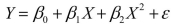where Y = demand (in thousands)and X = retail price per carat. 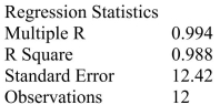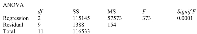This model was fit to data collected for a sample of 12 rare gems of this type.A portion of the computer analysis obtained from Microsoft Excel is shown below: SUMMARY OUTPUT 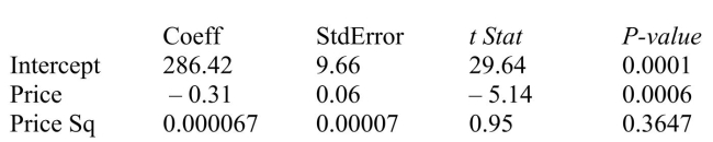-Referring to Scenario 15-1, what is the correct interpretation of the coefficient of multiple determination?

Two simple regression models were used to predict a single dependent variable.Both models were highly significant, but when the two independent variables were placed in the same multiple regression model for the dependent variable, did not increase substantially and the parameter estimates for the model were not significantly different from 0.This is probably an example of collinearity.

As a project for his business statistics class, a student examined the factors that determined parking meter rates throughout the campus area.Data were collected for the price per hour of parking, blocks to the quadrangle, and one of the three jurisdictions: on campus, in downtown and off campus, or outside of downtown and off campus.The population regression model hypothesized is 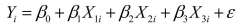where Y is the meter price is the number of blocks to the quad is a dummy variable that takes the value 1 if the meter is located in downtown and off campus and the value 0 otherwise is a dummy variable that takes the value 1 if the meter is located outside of downtown and off campus, and the value 0 otherwise Suppose that whether the meter is located on campus is an important explanatory factor. Why should the variable that depicts this attribute not be included in the model?

With four independent variables in a proposed regression model, how many models would need to be evaluated in a best subsets approach?

SCENARIO 15-4 The superintendent of a school district wanted to predict the percentage of students passing a sixth-grade proficiency test.She obtained the data on percentage of students passing the proficiency test (% Passing), daily mean of the percentage of students attending class (% Attendance), mean teacher salary in dollars (Salaries), and instructional spending per pupil in dollars (Spending)of 47 schools in the state. Let Y = % Passing as the dependent variable, Attendance, Salaries and Spending. The coefficient of multiple determination ( )of each of the 3 predictors with all the other remaining predictors are, respectively, 0.0338, 0.4669, and 0.4743. The output from the best-subset regressions is given below: Following is the residual plot for % Attendance: Following is the output of several multiple regression models: -Referring to Scenario 15-4, the "best" model chosen using the adjusted R-square statistic is

SCENARIO 15-1 A certain type of rare gem serves as a status symbol for many of its owners.In theory, for low prices, the demand increases, and it decreases as the price of the gem increases.However, experts hypothesize that when the gem is valued at very high prices, the demand increases with price due to the status owners believe they gain in obtaining the gem.Thus, the model proposed to best explain the demand for the gem by its price is the quadratic model: where Y = demand (in thousands)and X = retail price per carat. This model was fit to data collected for a sample of 12 rare gems of this type.A portion of the computer analysis obtained from Microsoft Excel is shown below: SUMMARY OUTPUT -Referring to Scenario 15-1, a more parsimonious simple linear model is likely to be statistically superior to the fitted curvilinear for predicting sale price (Y).

SCENARIO 15-6 Given below are results from the regression analysis on 40 observations where the dependent variable is the number of weeks a worker is unemployed due to a layoff (Y)and the independent variables are the age of the worker ( ), the number of years of education received ( ), the number of years at the previous job ( ), a dummy variable for marital status ( 1 = married, 0 = otherwise), a dummy variable for head of household ( 1 = yes, 0 = no)and a dummy variable for management position ( 1 = yes, 0 = no). The coefficient of multiple determination ( )for the regression model using each of the 6 variables as the dependent variable and all other X variables as independent variables are, respectively, 0.2628, 0.1240, 0.2404, 0.3510, 0.3342 and 0.0993. The partial results from best-subset regression are given below: -Referring to Scenario 15-6, what is the value of the variance inflationary factor of Job Yr?