Exam 16: Time-Series Forecasting

SCENARIO 16-13 Given below is the monthly time series data for U.S.retail sales of building materials over a specific year. 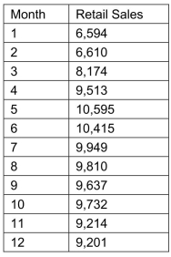The results of the linear trend, quadratic trend, exponential trend, first-order autoregressive, second-order autoregressive and third-order autoregressive model are presented below in which the coded month for the month is 0: 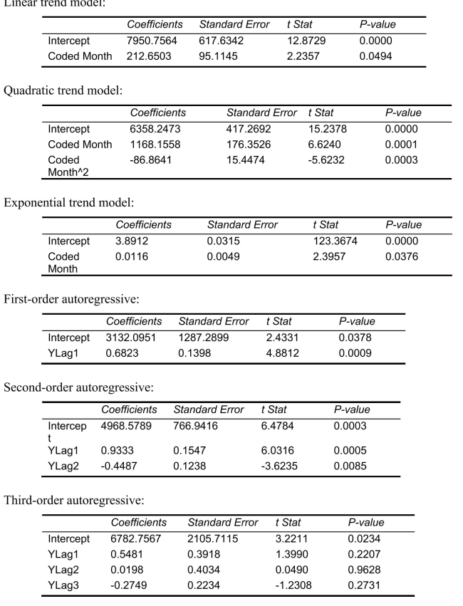Below is the residual plot of the various models: 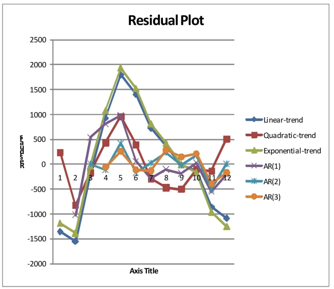-Referring to Scenario 16-13, what is the exponentially smoothed value for the 1 month using a smoothing coefficient of W = 0.5 if the exponentially smooth value for the 1 and 1 month are 9,746.3672 and 9,480.1836, respectively?

The overall upward or downward pattern of the data in an annual time series will be contained in the ____________ component.

After estimating a trend model for annual time-series data, you obtain the following residual plot against time, the problem with your model is that:

SCENARIO 16-10 Business closures in a city in the western U.S.from 2007 to 2012 were: 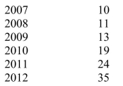Microsoft Excel was used to fit both first-order and second-order autoregressive models, resulting in the following partial outputs: 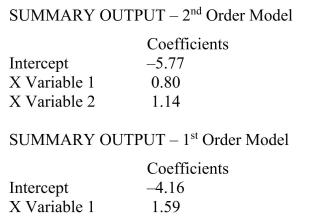-Referring to Scenario 16-10, the fitted values for the first-order autoregressive model are ________, ________, ________, ________, and ________.

A least squares linear trend line is just a simple regression line with the years recoded.

If a time series does not exhibit a long-term trend, the method of exponential smoothing may be used to obtain short-term predictions about the future.

SCENARIO 16-14 A contractor developed a multiplicative time-series model to forecast the number of contracts in future quarters, using quarterly data on number of contracts during the 3-year period from 2011 to 2013.The following is the resulting regression equation: where is the estimated number of contracts in a quarter. X is the coded quarterly value with X = 0 in the first quarter of 2011. is a dummy variable equal to 1 in the first quarter of a year and 0 otherwise. Q is a dummy variable equal to 1 in the second quarter of a year and 0 otherwise. is a dummy variable equal to 1 in the third quarter of a year and 0 otherwise. -Referring to Scenario 16-14 , the best interpretation of the constant 3.37 in the regression equation is:

In selecting a forecasting model, you should perform a residual analysis.

SCENARIO 16-12 A local store developed a multiplicative time-series model to forecast its revenues in future quarters, using quarterly data on its revenues during the 5-year period from 2009 to 2013.The following is the resulting regression equation: where is the estimated number of contracts in a quarter. X is the coded quarterly value with X = 0 in the first quarter of 2008. is a dummy variable equal to 1 in the first quarter of a year and 0 otherwise. is a dummy variable equal to 1 in the second quarter of a year and 0 otherwise. is a dummy variable equal to 1 in the third quarter of a year and 0 otherwise. -Referring to Scenario 16-12, the estimated quarterly compound growth rate in revenues is around:

SCENARIO 16-5 The number of passengers arriving at San Francisco on the Amtrak cross-country express on 6 successive Mondays were: 60, 72, 96, 84, 36, and 48. -Referring to Scenario 16-5, the number of arrivals will be smoothed with a 3-term moving average.The first smoothed value will be __________.

SCENARIO 16-13 Given below is the monthly time series data for U.S.retail sales of building materials over a specific year. The results of the linear trend, quadratic trend, exponential trend, first-order autoregressive, second-order autoregressive and third-order autoregressive model are presented below in which the coded month for the month is 0: Below is the residual plot of the various models: -Referring to Scenario 16-13, if a five-month moving average is used to smooth this series, what would be the first calculated value?

SCENARIO 16-8 The manager of a marketing consulting firm has been examining his company's yearly profits. He believes that these profits have been showing a quadratic trend since 1994.He uses Microsoft Excel to obtain the partial output below.The dependent variable is profit (in thousands of dollars), while the independent variables are coded years and squared of coded years, where 1994 is coded as 0, 1995 is coded as 1, etc. SUMMARY OUTPUT 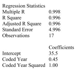-Referring to Scenario 16-8, the forecast for profits in 2014 is __________.

SCENARIO 16-12 A local store developed a multiplicative time-series model to forecast its revenues in future quarters, using quarterly data on its revenues during the 5-year period from 2009 to 2013.The following is the resulting regression equation: where is the estimated number of contracts in a quarter. X is the coded quarterly value with X = 0 in the first quarter of 2008. is a dummy variable equal to 1 in the first quarter of a year and 0 otherwise. is a dummy variable equal to 1 in the second quarter of a year and 0 otherwise. is a dummy variable equal to 1 in the third quarter of a year and 0 otherwise. -Referring to Scenario 16-12, using the regression equation, what is the forecast for the revenues in the third quarter of 2014?

Given a data set with 15 yearly observations, there are only seven 9-year moving averages.

SCENARIO 16-6 The president of a chain of department stores believes that her stores' total sales have been showing a linear trend since 1993.She uses Microsoft Excel to obtain the partial output below. The dependent variable is sales (in millions of dollars), while the independent variable is coded years, where 1993 is coded as 0, 1994 is coded as 1, etc. SUMMARY OUTPUT 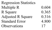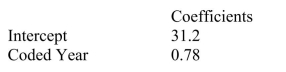-Referring to Scenario 16-6, the fitted trend value (in millions of dollars)for 1993 is __________.

SCENARIO 16-4 The number of cases of merlot wine sold by a Paso Robles winery in an 8-year period follows. 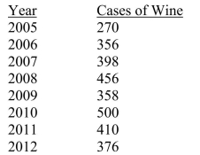-Referring to Scenario 16-4, construct a centered 3-year moving average for the wine sales.

SCENARIO 16-9 Given below are EXCEL outputs for various estimated autoregressive models for a company's real operating revenues (in billions of dollars)from 1989 to 2012.From the data, you also know that the real operating revenues for 2010, 2011, and 2012 are 11.7909, 11.7757 and 11.5537, respectively. 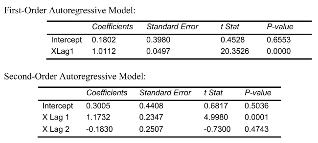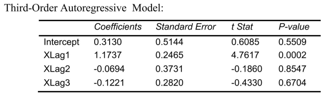-Referring to Scenario 16-9 and using a 5% level of significance, what is the appropriate autoregressive model for the company's real operating revenue?

SCENARIO 16-13 Given below is the monthly time series data for U.S.retail sales of building materials over a specific year. The results of the linear trend, quadratic trend, exponential trend, first-order autoregressive, second-order autoregressive and third-order autoregressive model are presented below in which the coded month for the month is 0: Below is the residual plot of the various models: -Referring to Scenario 16-13, you can conclude that the quadratic term in the quadratic-trend model is statistically significant at the 5% level of significance.

SCENARIO 16-4 The number of cases of merlot wine sold by a Paso Robles winery in an 8-year period follows. -Referring to Scenario 16-4, exponentially smooth the wine sales with a weight or smoothing constant of 0.4.

SCENARIO 16-11 The manager of a health club has recorded mean attendance in newly introduced step classes over the last 15 months: 32.1, 39.5, 40.3, 46.0, 65.2, 73.1, 83.7, 106.8, 118.0, 133.1, 163.3, 182.8, 205.6, 249.1, and 263.5.She then used Microsoft Excel to obtain the following partial output for both a first- and second-order autoregressive model. SUMMARY OUTPUT - Order Model 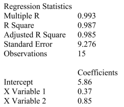SUMMARY OUTPUT - 1 Order Model 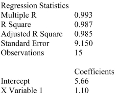-Referring to Scenario 16-11, based on the parsimony principle, the second- order model is the better model for making forecasts.