Exam 18: Time Series and Forecasting

Which of the following is not based on a regression model?

When the decomposition model, y_t = T_t × S_t × I_t, is applied, forecasts are made as = + , where represents the estimated trend for seasonally adjusted time series for period t, and is the seasonal index for period t.

Based on quarterly data collected over the last four years, the following regression equation was found to forecast the quarterly demand for the number of new copies of an economics textbook: _t = 3,305 - 665Qtr1 - 1,335Qtr2 + 305Qtr3, where Qtr1, Qtr2, and Qtr3 are dummy variables corresponding to Quarters 1, 2, and 3. By what percent is the demand in Quarter 3 higher on average than the average quarterly demand?

Which of the following types of trend models will best suit a series where the value of the series changes by a fixed amount for each period?

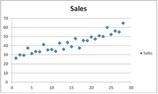
The following table shows the annual revenues (in millions of dollars) of a pharmaceutical company over the period 1990-2011. 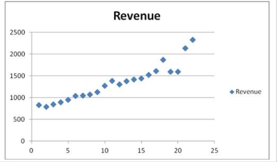The scatterplot indicates that the annual revenues have an increasing trend. Linear, exponential, quadratic, and cubic models were fit to the data starting with t = 1, and the following output was generated. When all four trend regression equations are compared, which of them provides the best fit?

Prices of crude oil have been steadily rising over the last two years (The Wall Street Journal, December 14, 2010). The monthly data on price per gallon of unleaded regular gasoline in the United States from January 2009 to December 2010 were available. Three trend models were created starting with t = 1, and the following output was generated. Based on adjusted R², which of the following models is the most appropriate for making a forecast for the price of regular unleaded gasoline?

The ________ is a trend model that allows for one change in the direction of a series.

The past monthly demands are shown below. The naïve method, that is, the one-period moving average method, is applied to make forecasts. 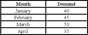What is the mean absolute deviation (MAD) of the forecasts?

The seasonal component typically represents repetitions over a ________ period.

Which of the following types of trend models will best suit a series where the increase in value of the series gets larger over time?

Which of the following equations is a one-period-ahead forecast of the autoregressive model AR(1)?

The mean of the absolute residuals defines the ________.

The following table includes the information about a monthly time series. 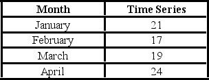When the exponential smoothing method with α = 0.1 and α = 0.5 is applied, what is the speed of decline for which the mean square error is better? What is this mean?

When using Excel for calculating moving averages, the Moving Average dialog box should be activated. The value of m - the number of periods should be entered in the box named ________.

The ________ of the adjusted seasonal indices equals one.

In a moving average method, when a new observation becomes available, the new average is computed by including the new observation and ________.

Quarterly sales of a department store for the last seven years are given in the following table. 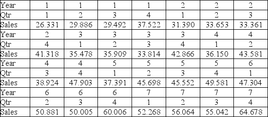The scatterplot shows that the quarterly sales have an increasing trend and seasonality. A linear regression model given by Sales = β₀ + β₁Qtr1 + β₂Qtr2 + β₃Qtr3 + β₄t + ε, where t is the time period (t = 1, ..., 28) and Qtr1, Qtr2, and Qtr3 are quarter dummies, is estimated and then used to make forecasts. For the regression model, the following partial output is available. Using the regression equation for the linear trend model with seasonal dummy variables, what is the sales forecast for the first quarter of Year 8?

Although we use the MSE to compare the linear and the exponential trend models, we cannot use it to compare the linear, quadratic, and cubic trend models.

The following table shows the annual revenues (in millions of dollars) of a pharmaceutical company over the period 1990-2011. 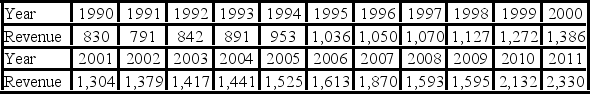The autoregressive models of order 1 and 2, y_t = β₀ + β₁y_{t - 1} + ε_t, and y_t = β₀ + β₁y_{t - 1} + β₂y_{t - 2} + ε_t, were applied on the time series to make revenue forecasts. The relevant parts of Excel regression outputs are given below. Model AR(1): Model AR(2): Using the AR(2) model, find the company revenue forecast for 2012.

Quarterly sales of a department store for the last seven years are given in the following table. The scatterplot shows that the quarterly sales have an increasing trend and seasonality. A linear regression model given by Sales = β₀ + β₁Qtr1 + β₂Qtr2 + β₃Qtr3 + β₄t + ε, where t is the time period (t = 1, ..., 28) and Qtr1, Qtr2, and Qtr3 are quarter dummies, is estimated and then used to make forecasts. For the regression model, the following partial output is available. Using MSE and MAD, compare the linear trend equation with seasonal dummy variables, _t = 31,9261 - 7.855Qtr1 - 4.7362Qtr2 - 7.1656Qtr3 + 1.0749t, and the decomposition method equation _t = _t × _t with t = 26.8819 + 1.0780t and the quarterly seasonal indices: 0.9322, 1.0066, 0.9441, and 1.1171. Which of the two corresponding forecasting models is recommended?