Exam 16: A: Simple Linear Regression and Correlation

The degrees of freedom for the test statistic for the slope is ____________________.

Grateful Dead Concert At a recent Grateful Dead concert,a survey was conducted that asked a random sample of 20 people their age and how many concerts they have attended since the first of the year.It is suspected that older concert goers tend to go to more of his concerts in one year than younger concert goers.The data and analysis are shown below. AEe 62 57 40 49 67 54 43 65 54 41 Number af Concerts 6 5 4 3 5 5 2 6 3 1 Age 44 48 55 60 59 63 69 40 38 52 Number of Concerts 3 2 4 5 4 5 4 2 1 3 An Excel output follows: 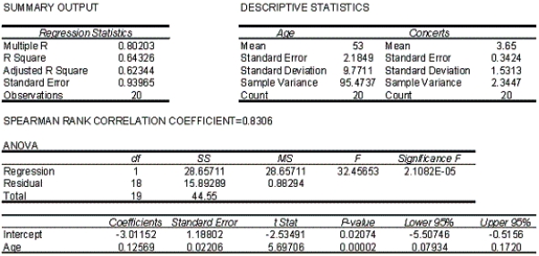-{Oil Quality and Price Narrative} Calculate the Pearson correlation coefficient.What sign does it have? Why?

In regression analysis,if the coefficient of determination is 1.0,then:

Income and Education A professor of economics wants to study the relationship between income (y in $1000s)and education (x in years).A random sample eight individuals is taken and the results are shown below. Education 16 11 15 8 12 10 13 14 Income 58 40 55 35 43 41 52 49 -{Income and Education Narrative} Interpret the value of the slope of the regression line.

In testing the hypotheses: H₀: $\beta$ ₁ = 0 vs.H₀: $\beta$ ₁ $\neq$ 0,the following statistics are available: $n = 10$ , $b _ { 0 } = - 1.8$ , $b _ { 1 } = 2.45$ , $s _ { ? _ { 1 } } = 1.20$ ,and $\hat { y } = 6$ .The value of the test statistic is:

A confidence interval (as opposed to a prediction interval)is used to estimate the long-run average value of y.

The smallest value that the standard error of estimate s _{$\varepsilon$} can assume is:

Grateful Dead Concert At a recent Grateful Dead concert,a survey was conducted that asked a random sample of 20 people their age and how many concerts they have attended since the first of the year.It is suspected that older concert goers tend to go to more of his concerts in one year than younger concert goers.The data and analysis are shown below. AEe 62 57 40 49 67 54 43 65 54 41 Number af Concerts 6 5 4 3 5 5 2 6 3 1 Age 44 48 55 60 59 63 69 40 38 52 Number of Concerts 3 2 4 5 4 5 4 2 1 3 An Excel output follows: -{Grateful Dead Concert Narrative} Determine the coefficient of determination and discuss what its value tells you about the two variables.

Suppose the slope of a simple linear regression line between hours studying and exam score is 5.That means as ____________________ increases by one,____________________ increases by 5.

Oil Quality and Price Quality of oil is measured in API gravity degrees--the higher the degrees API,the higher the quality.The table shown below is produced by an expert in the field who believes that there is a relationship between quality and price per barrel. $\begin{array} { | c | c | } \hline \text { Oi degrees API } & \text { Price per barrel (in \$) } \\\hline 27.0 & 12.02 \\28.5 & 12.04 \\30.8 & 12.32 \\31.3 & 12.27 \\31.9 & 12.49 \\34.5 & 12.70 \\34.0 & 12.80 \\34.7 & 13.00 \\37.0 & 13.00 \\41.0 & 13.17 \\41.0 & 13.19 \\38.8 & 13.22 \\39.3 & 13.27 \\\hline\end{array}$ A partial Minitab output follows: Dascriptive atafistics Variable Mear StDev SE Mear Degrees 13 34.60 4.613 1.280 Price 13 1270 0.757 0.127 Covariances Degeres Price Degeres 21.281667 Price 2.026750 0.208933 Analysis of Variance Source DF SS MS F p Regeression 1 2.3162 2.3162 134.24 0.000 Resichul Entar 11 0.1898 0.0173 Total 12 2.5060 -{Oil Quality and Price Narrative} Draw a scatter diagram of the data.Comment on whether it appears that a linear model might be appropriate to describe the relationship between the quality of oil and price per barrel.

Statisticians have shown that sample y-intercept b₀ and sample slope coefficient b₁ are unbiased estimators of the population regression parameters $\beta$ ₀ and $\beta$ ₁,respectively.

Rock Concert Revenues A financier whose specialty is investing in rock concerts has observed that,in general,concerts with "big-name" stars seem to generate more revenue than those concerts whose stars are less well known.To examine his belief he records the gross revenue and the payment (in $ millions)given to the two highest-paid performers in the concert for ten concert tours. Concert Cost of Twa Highest Paid Perfarmers ( \mil ) Grass Revenue () 1 5.3 48 2 7.2 65 3 1.3 18 4 1.8 20 5 3.5 31 6 2.6 26 7 8.0 73 8 2.4 23 9 4.5 39 10 0.7 58 -{Rock Concert Revenues Narrative} Determine the standard error of estimate and describe what this statistic tells you about the regression line.

Grateful Dead Concert At a recent Grateful Dead concert,a survey was conducted that asked a random sample of 20 people their age and how many concerts they have attended since the first of the year.It is suspected that older concert goers tend to go to more of his concerts in one year than younger concert goers.The data and analysis are shown below. AEe 62 57 40 49 67 54 43 65 54 41 Number af Concerts 6 5 4 3 5 5 2 6 3 1 Age 44 48 55 60 59 63 69 40 38 52 Number of Concerts 3 2 4 5 4 5 4 2 1 3 An Excel output follows: -{Oil Quality and Price Narrative} Do the $\rho$ and $\beta$ ₁ tests in the previous two questions provide the same results? Explain.

An inverse relationship between an independent variable x and a dependent variably y means that as x increases,y decreases,and vice versa.

Accidents and Rain A statistician investigating the relationship between the amount of rain (in inches)and the number of automobile accidents gathered data on accidents in her city for 10 randomly selected days throughout the year.The results are shown below. Day Rain Number of Accidents 1 0.05 5 2 0.12 6 3 0.05 2 4 0.08 4 5 0.10 6 0.35 14 7 0.15 7 8 0.30 13 9 0.10 7 10 0.20 10 -{Accidents and Rain Narrative} Find the least squares regression line.

Truck Speed and Gas Mileage An economist wanted to analyze the relationship between the speed of a truck (x)and its gas mileage (y).As an experiment a truck is operated at several different speeds and for each speed the gas mileage is measured.These data are shown below. Speed 25 35 45 50 60 65 70 Gas Mileage 40 39 37 33 30 27 25 -{Truck Speed and Gas Mileage Narrative} Predict with 99% confidence the gas mileage of a car traveling 55 mph.

Allman Brothers Concert At a recent Allman Brothers concert,a survey was conducted that asked a random sample of 20 people their age and how many concerts they have attended since the first of the year.The following data were collected: Age 62 57 40 49 67 54 43 65 54 41 Number af Concerts 6 5 4 3 5 5 2 6 3 1 Age 44 48 55 60 59 63 69 40 38 52 Number af Concerts 3 2 4 5 4 5 4 2 1 3 An Excel output follows: 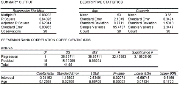-{Allman Brothers Concert Narrative} Plot the least squares regression line on the scatter diagram.

The coefficient of ____________________ measures the amount of variation in the dependent variable that is explained by the variation in the independent variable.

Sunshine and Melanoma A medical researcher wanted to examine the relationship between the amount of sunshine (x)in hours,and incidence of melanoma,a type of skin cancer (y).As an experiment he found the number of melanoma cases detected per 100,000 of population and the average daily sunshine in eight counties around the country.These data are shown below. Average Daily Sunshine 5 7 6 7 8 6 4 3 Melanoma per 100,000 7 11 9 12 15 10 7 5 -{Sunshine and Melanoma Narrative} What does the value of the slope of the regression line tell you?

A regression analysis between sales (in $1000)and advertising (in $100)resulted in the following least squares line: $\hat { y } = 75 + 6 x$ .This implies that if advertising is $800,then the predicted amount of sales (in dollars)is: