Exam 17: Time Series Forecasting and Index Numbers

Consider the quarterly production data (in thousands of units) for the XYZ manufacturing company below. The normalized (adjusted) seasonal factors are winter = .9982, spring = .9263, summer = 1.139, and fall = .9365. Calculate the deseasonalized production value for each observation in the time series.

Consider the regression equation = 18.321 + 3.762(t) and the data below. 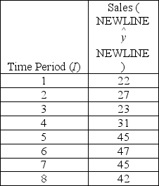Compute the residuals (error terms) for periods 6 and 7.

The no-trend time series model is given by

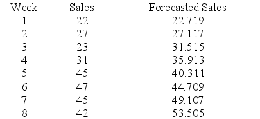
Consider the regression equation = 6.04 + .10 (t) and the data below. Compute the predicted value of sales for period 8.

Consider the following data and calculate S₁ using simple exponential smoothing and α = .3.

The demand for a product for the last six years has been 15, 15, 17, 18, 20, and 19. The manager wants to predict the demand for this time series using the following simple linear trend equation: tr_t = 12 + 2t. What are the forecast errors for the 5th and 6th years?

The upward or downward movement that characterizes a time series over a period of time is referred to as ________.

Holt-Winters double exponential smoothing would be an appropriate method to use to forecast a time series that exhibits a linear trend with no seasonal or cyclical patterns.

The linear trend equation for the following data is = 1.4286 + 2.5(t). What is the predicted value of the fund in the period t = 1?

Consider the following set of quarterly sales data, given in thousands of dollars. The following dummy variable model that incorporates a linear trend and constant seasonal variation was used: y(t) = β₀ + β_1t + β_Q1(Q1) + β_Q2(Q2) + β_Q3(Q3) + E_t. In this model, there are three binary seasonal variables (Q1, Q2, and Q3), where Qi is a binary (0,1) variable defined as: Qi = 1, if the time series data is associated with quarter i; Qi = 0, if the time series data is not associated with quarter i. The results associated with this data and model are given in the following Minitab computer output. The regression equation is Sales = 2442 + 6.2 Time − 693 Q1 − 1499 Q2 + 153 Q3 Analysis of Variance Provide a managerial interpretation of the regression coefficients for the variables Q1 (quarter 1), Q2 (quarter 2), and Q3 (quarter 3).

The multiplicative Winters method used to forecast time series applies a seasonal factor SN_T to the forecasting model.

Which of the following is not a component of time series?

Consider a time series with 15 quarterly sales observations. Using the quadratic trend model, the following partial computer output was obtained. What is the predicted value of y when t = 20?

The linear regression trend model was applied to a time series of sales data based on the last 16 months of sales. The following partial computer output was obtained. Write the prediction equation.

A simple exponential forecasting method would not be used to forecast seasonal data.

The Durbin-Watson statistic is used to detect ________.

Given the following data, compute the mean absolute deviation.

If the errors produced by a forecasting method for 3 observations are +3, +3, and −3, then what is the mean squared error?

Cyclical variation exists when the magnitude of the seasonal swing does not depend on the level of a time series.

While a simple index is calculated by using the values of one time series, an aggregate index is computed based on the accumulated values of more than one time series.