Exam 17: Time Series Forecasting and Index Numbers

Forecasters using a multiplicative decomposition model or time series regression model, assume that the time series components are changing over time.

The following data on prices and quantities for the years 1995 and 2000 are given for three products. Calculate the 2000 Paasche index.

Consider a time series with 15 quarterly sales observations. Using the quadratic trend model, the following partial computer output was obtained. Test the significance of the t² term at α =.05. State the critical T value (rejection point) and the p-value. Make your decision using a two-sided null hypothesis.

Those fluctuations that are associated with climate, holidays, and related activities are referred to as ________ variations.

When deseasonalizing a time series observation, we divide the actual time series observation by its ________.

Exponential smoothing is designed to forecast time series described by regular and seasonal components that are always changing over time.

When preparing a price index based on multiple products, if the price of each product is weighted by the quantity of the product purchased in a given period of time, the resulting index is called a ________ price index.

Consider the quarterly production data (in thousands of units) for the XYZ manufacturing company below. The normalized (adjusted) seasonal factors are winter = .9982, spring = .9263, summer = 1.139, and fall = .9365. Based on the following deseasonalized observations (d_t), a trend line was estimated. 1998 1999 2000 The following Minitab output gives the straight-line trend equation fitted to the deseasonalized observations. Based on the trend equation given below, calculate the trend value for each period in the time series. The regression equation is Deseasonalized = 10.1 + 1.91 × Time

Simple exponential smoothing is a forecasting method that applies equal weights to the time series observations.

A forecasting method that weights recent observations more heavily is called ________.

When there is ________ seasonal variation, the magnitude of the seasonal swing does not depend on the level of the time series.

Consider the following set of quarterly sales data, given in thousands of dollars. The following dummy variable model that incorporates a linear trend and constant seasonal variation was used: y(t) = β₀ + β_1t + β_Q1(Q1) + β_Q2(Q2) + β_Q3(Q3) + E_t. In this model, there are three binary seasonal variables (Q1, Q2, and Q3), where Qi is a binary (0,1) variable defined as: Qi = 1, if the time series data is associated with quarter i; Qi = 0, if the time series data is not associated with quarter i. The results associated with this data and model are given in the following Minitab computer output. The regression equation is Sales = 2442 + 6.2 Time − 693 Q1 − 1499 Q2 + 153 Q3 Analysis of Variance Provide a managerial interpretation of the regression coefficient for the variable "time."

The Box-Jenkins methodology can be used to identify what is called an autoregressive-moving average model.

XYZ Company, Annual Data Based on the information given in the table above, we can conclude that, in general,

A positive autocorrelation implies that negative error terms will be followed by ________ error terms.

The multiplicative Winters method is used to forecast time series when there are no seasonal factors that are part of the model.

The following data on prices and quantities for the years 1995 and 2000 are given for three products. Calculate the 2000 Laspeyres index.

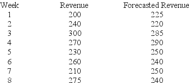
Given the following data, compute the total error (sum of the error terms).

Two forecasting models were used to predict the future values of a time series. The forecasts are shown below with the actual values. Calculate the mean absolute deviation (MAD) for Model 1.

Dummy variables are used to model increasing seasonal variation.