Exam 17: Time Series Forecasting and Index Numbers

A restaurant has been experiencing higher sales during the weekends, compared to the weekdays. Daily restaurant sales patterns for this restaurant over a week are an example of a(n) ________ component of a time series.

The following data on prices and quantities for the years 1995 and 2000 are given for three products. Calculate the 2000 aggregate price index.

The purpose behind moving averages and centered moving averages is to eliminate ________.

When using simple exponential smoothing, the value of the smoothing constant α cannot be

A positive autocorrelation implies that negative error terms will be followed by negative error terms.

Two forecasting models were used to predict the future values of a time series. The forecasts are shown below with the actual values. Calculate the mean squared deviation (MSD) for Model 1.

The Laspeyres index and the Paasche index are both examples of ________ aggregate price indexes.

Given the following data, compute the mean absolute deviation (MAD).

A univariate time series model is used to predict future values of a time series based only upon past values of a time series.

The smoothing constant is a number that determines how much weight is attached to each observation.

Given the following data, compute the mean absolute deviation.

The price and quantity of several food items are listed below for the years 1990 and 2000. Compute the Laspeyres index, using 1990 as the base year.

Consider the following data. Calculate S₁ using simple exponential smoothing and α = .2.

Use the following price information for three grains. Calculate the simple price index for each grain separately.

XYZ Company, Annual Data Based on the information given in the table above, what is the MAD?

Seasonal variations are periodic patterns in a time series that are repeated over time. For which one of the following time series variables is it not possible to recognize seasonal variations?

Consider the following set of quarterly sales data, given in thousands of dollars. The following dummy variable model that incorporates a linear trend and constant seasonal variation was used: y(t) = β₀ + β_1t + β_Q1(Q1) + β_Q2(Q2) + β_Q3(Q3) + E_t. In this model, there are three binary seasonal variables (Q1, Q2, and Q3), where Qi is a binary (0,1) variable defined as: Qi = 1, if the time series data is associated with quarter i; Qi = 0, if the time series data is not associated with quarter i. The results associated with this data and model are given in the following Minitab computer output. The regression equation is Sales = 2442 + 6.2 Time − 693 Q1 − 1499 Q2 + 153 Q3 Analysis of Variance At α = .05, test the significance of the model.

Consider the regression equation = 18.321 + 3.762(t) and the data below. 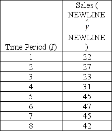Compute the predicted value for sales for periods 6 and 7.

A simple index is obtained by dividing the current value of a time series by the value of a time series in the ________ time period and by multiplying this ratio by 100.

Assume that the current date is February 1, 2003. The linear regression model was applied to a monthly time series based on the last 24 months' sales (from January 2000 through December 2002). The following partial computer output summarizes the results. Determine the predicted sales for this month.