Exam 2: Exploring Relationships Between Variables

Which is true? I. Random scatter in the residuals indicates a model with high predictive power. II. If two variables are very strongly associated, then the correlation between them will be near +1.0 Or -1.0. III. The higher the correlation between two variables the more likely the association is based in Cause and effect.

After conducting a marketing study to see what consumers thought about a new tinted contact lens they were developing, an eyewear company reported, "Consumer satisfaction is strongly correlated with eye color." Comment on this observation.

A study by a prominent psychologist found a moderately strong positive association between the number of hours of sleep a person gets and the person's ability to memorize information. a. Explain in the context of this problem what "positive association" means. b. Hoping to improve academic performance, the psychologist recommended the school board allow students to take a nap prior to any assessment. Discuss the psychologist's recommendations.

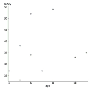
Halloween is a fun night. It seems that older children might get more candy because they can travel further while trick-or-treating. But perhaps the youngest kids get extra candy because they are so cute. Here are some data that examine this question, along with the regression output. Dependent Variable: candy Sample size: 9 $R$ (correlation coefficient) $= \mathbf { 0 . 1 9 5 3 4 4 2 5 }$ $\mathrm { R } - \mathrm { sq } = 0.038159375$ $s = 11.297554$ Parameter Estimate Std. Err. Intercept 13.569231 9.0783516 Age 3.4038462 1.0175376 -The next day, a young girl reveals that her older brother also went trick-or-treating, but didn't want to admit that he participated. He was added to the data set and these are the results. Dependent Variable: candy Sample size: 10 $R$ (correlation coefficient $) = 0.76362369$ $\mathrm { R } - \mathrm { sq } = 0.58312115$ $\mathrm { s } = 12.709041$ Parameter Estimate Std. Err. Intercept 13.569231 9.0783516 Age 3.4038462 1.0175376 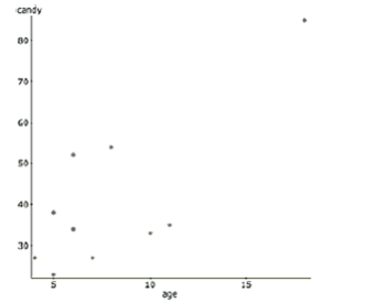Describe the effect of this new candy collector on the regression model.

A common objective for many school administrators is to increase the number of students taking SAT and ACT tests from their school. The data from each state from 2003 are reflected in the scatterplot. 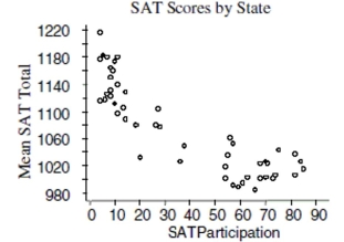a. Write a few sentences describing the association. b. Estimate the correlation. $r =$ __________ c. If the point in the top left corner (4, 1215) were removed, would the correlation become stronger, weaker, or remain about the same? Explain briefly. d. If the point in the very middle (38, 1049) were removed, would the correlation become stronger, weaker, or remain about the same? Explain briefly.

Associations For each pair of variables, indicate what association you expect: positive(+), $\text { negative } ( - ) \text {, curved } ( \mathrm { C } ) \text {, or none } ( \mathrm { N } ) \text {. }$ a. power level setting of a microwave; number of minutes it takes to boil water b. number of days it rained in a month (during the summer); number of times you mowed your lawn that month c. number of hours a person has been up past a normal bedtime; number of minutes it takes the person to do a crossword puzzle d. number of hockey games played in Minnesota during a week; sales of suntan lotion in Minnesota during that week e. length of a student's hair; number of credits the student earned last year

Earning power A college's job placement office collected data about students' GPAs and the salaries they earned in their first jobs after graduation. The mean GPA was 2.9 with a standard deviation of 0.4. Starting salaries had a mean of $47,200 with a SD of $8500. The correlation between the two variables was $r = 0.72$ The association appeared to be linear in the scatterplot. (Show work) a. Write an equation of the model that can predict salary based on GPA. b. Do you think these predictions will be reliable? Explain. c. Your brother just graduated from that college with a GPA of 3.30. He tells you that based on this model the residual for his pay is -$1880. What salary is he earning?

Math and Verbal Suppose the correlation between SAT Verbal scores and Math scores is 0.57 and that these scores are normally distributed. If a student's Verbal score places her at the 90th percentile, at what percentile would you predict her Math score to be? (SHOW WORK)

Which of the following is not a source of caution in regression between two variables?

The correlation coefficient between high school grade point average (GPA) and college GPA is 0)560. For a student with a high school GPA that is 2.5 standard deviations above the mean, we Would expect that student to have a college GPA that is ______ the mean.

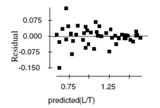
To achieve linearity, the data was transformed using a square root function of cost. Here are the results and a residual plot. Dependent Variable: sqrt(cost) s: $0.2141$ Parameter coeff se Intercept 1.1857 0.4346 height 0.1792 0.0151 -Interpret R-sq in the context of this problem.

A regression analysis of students' college grade point averages (GPAs) and their high school GPAs Found $R ^ { 2 } = 0.311$ 11) Which of these is true? I. High school GPA accounts for 31.1% of college GPA. II. 31.1% of college GPAs can be correctly predicted with this model. III. 31.1% of the variance in college GPA can be accounted for by the model

You are given the following costs to build a square deck for your house: $\begin{array} { | l | c | c | c | c | c | c | c | c | c | c | c | c | } \hline \text { Width (ft) } & 4 & 5 & 6 & 7 & 8 & 9 & 10 & 11 & 12 & 13 & 14 & 15 \\\hline \text { Cost (\$) } & 150 & 255 & 350 & 500 & 650 & 800 & 1000 & 1200 & 1450 & 1700 & 1950 & 2250 \\\hline\end{array}$ a. Use re-expressed data to create a model that predicts the cost of the deck based on the width. b. Why do you think that your model is appropriate? c. Find the predicted cost of a square deck that is 10.5 feet wide. d. Is it reasonable to use this model to predict the cost of a square deck that is 20 feet wide? Explain.

During a science lab, students heated water, allowed it to cool, and recorded the temperature over time. They computed the difference between the water temperature and the room temperature. The results are in the table. Time (in minutes) 10 20 30 40 50 60 Difference in temp. (degrees F) 68 36 20 10 6 4 -Would it be better for customers for a year to have a negative residual or a positive residual from this model? Explain.

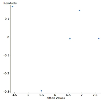
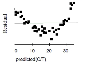
The residuals plot for a linear model is shown. Which is true?

After conducting a survey of his students, a professor reported that "There appears to be a strong correlation between grade point average and whether or not a student works." Comment on this observation.

Penicillin Doctors studying how the human body assimilates medication inject some patients with penicillin, and then monitor the concentration of the drug (in units/cc) in the patients' blood for seven hours. The data are shown in the scatterplot. First they tried to fit a linear model. The regression analysis and residuals plot are shown. Dependent variable is: Concentration No Selector R squared $= 90.8 \% \quad$ R squared (adjusted) $= 90.6 \%$ $s = 3.472$ with $43 - 2 = 41$ degrees of freedom Source Sum of Squares df Mean Square F-ratio Regression 4900.55 1 4900.55 407 Residual 494.199 41 12.0536 Variable Coefficient s.e. of Coeff t-ratio prob Constant 40.3266 1.295 31.1 \leq0.0001 Time -5.95956 0.2956 -20.2 \leq0.0001 a. Find the correlation between time and concentration. b. Using this model, estimate what the concentration of penicillin will be after 4 hours. c. Is that estimate likely to be accurate, too low, or too high? Explain. Now the researchers try a new model, using the re-expression log(Concentration). Examine the regression analysis and the residuals plot below. Dependent variable is: LogCnn No Selector R squared $= 98.0 \% \quad$ R squared (adjusted) $= 98.0 \%$ $s = 0.0451$ with $43 - 2 = 41$ degrees of freedom Source Sum of Squares df Mean Square F-ratio Regression 4.11395 1 4.11395 2022 Residual 0.083412 41 0.002034 Variable Coefficient s.e. of Coeff t-ratio prob Constant 1.80184 0.0168 107 \leq0.0001 Time -0.172672 0.0038 -45.0 \leq0.0001 d. Explain why you think this model is better than the original linear model. e. Using this new model, estimate the concentration of penicillin after 4 hours.

When using midterm exam scores to predict a student's final grade in a class, the student would Prefer to have a

Put to Work Some students have to work part time jobs to pay for college expenses. A researcher examined the academic performance of students with jobs versus those without. He found a positive association between the number of hours worked and GPA. Explain what "positive association" means in this context.

Education research consistently shows that students from wealthier families tend to have higher SAT scores. The slope of the line that predicts SAT score from family income is 6.25 points per $1000, And the correlation between the variables is 0.48. Then the slope of the line that predicts family Income from SAT score (in $1000 per point) …