Exam 2: Exploring Relationships Between Variables
Exam 1: Exploring and Understanding Data125 Questions
Exam 2: Exploring Relationships Between Variables165 Questions
Exam 3: Gathering Data111 Questions
Exam 4: Randomness and Probability148 Questions
Exam 5: From the Data at Hand to the World at Large128 Questions
Exam 6: Accessing Associations Between Variables93 Questions
Exam 7: Inference When Variables Are Related25 Questions
Exam 8: Regression, Associations, and Predictive Modeling792 Questions
Select questions type
Here is a scatterplot of weight versus height for students in an introductory statistics class.
The men are coded as "1" and appear as circles in the scatterplot; the women are coded as
"2" and appear as squares in the scatterplot. 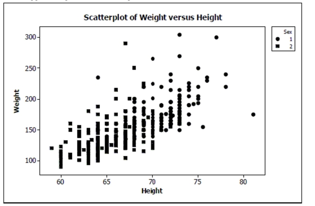 a. Do you think there is a clear pattern? Describe the association between weight and
height.
b. Comment on any differences you see between men and women in the plot.
c. Do you think a linear model from the set of all data could accurately predict the weight
of a student with height 70 inches? Explain.
a. Do you think there is a clear pattern? Describe the association between weight and
height.
b. Comment on any differences you see between men and women in the plot.
c. Do you think a linear model from the set of all data could accurately predict the weight
of a student with height 70 inches? Explain.
(Essay)
4.8/5  (36)
(36)
Baseball coaches use a radar gun to measure the speed of pitcher's fastball. They also record outcomes such as hits and
strikeouts. The scatterplot below shows the relationship between the average speed of a fastball and the average number of
strikeouts per nine innings for each pitcher on the Bulldogs, based on the past season. 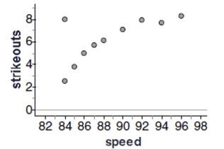 -Do you think a model based on these data could accurately predict the average number of
strikeouts for a pitcher with an average fastball speed of 70 mph.? Explain.
-Do you think a model based on these data could accurately predict the average number of
strikeouts for a pitcher with an average fastball speed of 70 mph.? Explain.
(Essay)
4.9/5 (34)
Another company's sales increase by the same percent each year. This growth is . . .
(Multiple Choice)
4.9/5 (31)
Which scatterplot shows a strong association between two variables even though the correlation is Probably near zero?
(Multiple Choice)
4.8/5 (35)
All but one of the statements below contain a mistake. Which one could be true?
(Multiple Choice)
4.8/5 (36)
Height and weight Suppose that both height and weight of adult men can be described
with Normal models, and that the correlation between these variables is 0.65. If a man's
height places him at the 60th percentile, at what percentile would you expect his weight to
be?
(Essay)
4.8/5 (43)
A residuals plot is useful because
I. it will help us to see whether our model is appropriate.
II. it might show a pattern in the data that was hard to see in the original scatterplot.
III. it will clearly identify influential points.
(Multiple Choice)
4.9/5 (44)
A correlation of zero between two quantitative variables means that
(Multiple Choice)
4.7/5 (45)
A regression equation is found that predicts the increased cost of a home owner's electricity bill
Given the number of holiday lights they put on the outside of their house. The equation is dol^lars =
2)5 + 0.02(light). If a house has 400 lights and a $15 increase in their electricity cost, find their
Residual.
(Multiple Choice)
4.9/5 (32)
A regression model examining the amount of weight a football player can bench press found that
10 cm differences in chest size are associated with 8 kg differences in weight pressed. Which is
True?
I. The correlation between chest size and weight pressed is
II. As a player gets stronger and presses more weight his chest will get bigger.
III. A positive residual means that the player pressed more than predicted.
(Multiple Choice)
4.8/5 (36)
An article in the Journal of Statistics Education reported the price of diamonds of different sizes in Singapore dollars (SGD).
The following table contains a data set that is consistent with this data, adjusted to US dollars in 2004: 2004 US \ Carat 494.82 0.12 768.03 0.17 1105.03 0.20 1508.88 0.25 1826.18 0.28 2096.89 0.33
2004 US \ Carat 688.24 0.15 944.90 0.18 1071.75 0.21 1504.44 0.26 1908.28 0.29 2409.76 0.35
2004 US \ Carat 748.10 0.16 1076.18 0.19 1289.20 0.23 1597.63 0.27 2038.09 0.32
-Do you think a linear model is appropriate here? Explain.
(Essay)
4.9/5 (39)
An article in the Journal of Statistics Education reported the price of diamonds of different sizes in Singapore dollars (SGD).
The following table contains a data set that is consistent with this data, adjusted to US dollars in 2004: 2004 US \ Carat 494.82 0.12 768.03 0.17 1105.03 0.20 1508.88 0.25 1826.18 0.28 2096.89 0.33
2004 US \ Carat 688.24 0.15 944.90 0.18 1071.75 0.21 1504.44 0.26 1908.28 0.29 2409.76 0.35
2004 US \ Carat 748.10 0.16 1076.18 0.19 1289.20 0.23 1597.63 0.27 2038.09 0.32
-Make a scatterplot and describe the association between the size of the diamond (carat) and
the cost (in US dollars).
(Essay)
5.0/5 (41)
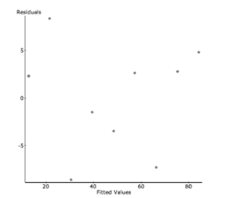
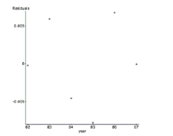
Shrimp From 1982 to 1990, there was a decrease in the number of white shrimp harvested
from the Galveston Bay. Here is the regression analysis and a residual plot. The year has
been shortened to two digits (82, 83…) and the dependent variable is the number of shrimp
collected per hour. Dependent Variable: Shrimp/hour
s:
Parameter Estimate Std. Err. constant 816.71111 66.903419 year -8.9333333 0.77759635
 a. Write the regression equation and define your variables.
b. Find the correlation coefficient and interpret it in context.
c. Interpret the value of the slope in context.
d. In 1991, the shrimp production rebounded (in part due to the effects of El Nino) to 81
shrimp/hour. Find the value of this residual.
e. The prediction for 1991 was very inaccurate. What name do statisticians give to this kind
of prediction error?
a. Write the regression equation and define your variables.
b. Find the correlation coefficient and interpret it in context.
c. Interpret the value of the slope in context.
d. In 1991, the shrimp production rebounded (in part due to the effects of El Nino) to 81
shrimp/hour. Find the value of this residual.
e. The prediction for 1991 was very inaccurate. What name do statisticians give to this kind
of prediction error?
(Essay)
4.8/5 (34)
During a chemistry lab, students were asked to study a radioactive element which decays
over time. The results are in the table. Time (in days) 0 2 4 6 8 10 Element (in grams) 320 226 160 115 80 57
a. Model the remaining mass of the element.
b. Find the predicted amount of the element remaining after thirty minutes.
(Essay)
4.8/5 (31)
Identify what is wrong with each of the following statements:
a. The correlation between Olympic gold medal times for the hurdles and year is seconds per year.
b. The correlation between Olympic gold medal times for the dash and year is . c. Since the correlation between Olympic gold medal times for the hurdles and dash is , the correlation between times for the dash and the hurdles is .
d. If we were to measure Olympic gold medal times for the hurdles in minutes instead of seconds, the correlation would be .
(Essay)
4.8/5 (32)
Students A growing school district tracks the student population growth over the years
from 2008 to 2013. Here are the regression results and a residual plot. students year
Sample size: 6
students y
Sample size: 6
R-sq
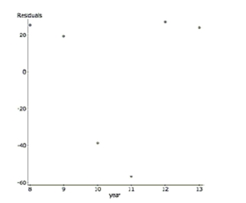 a. Explain why despite a high R-sq, this regression is not a successful model.
To linearize the data, the log (base 10) was taken of the student population. Here are the results.
Dependent Variable: log(students) Sample size: 6
Parameter Estimate Std. Err. constant 2.871 0.0162 year 0.0389 0.00152
a. Explain why despite a high R-sq, this regression is not a successful model.
To linearize the data, the log (base 10) was taken of the student population. Here are the results.
Dependent Variable: log(students) Sample size: 6
Parameter Estimate Std. Err. constant 2.871 0.0162 year 0.0389 0.00152
 b. Describe the success of the linearization.
c. Interpret R-sq in the context of this problem.
d. Predict the student population in 2014.
b. Describe the success of the linearization.
c. Interpret R-sq in the context of this problem.
d. Predict the student population in 2014.
(Essay)
4.9/5 (40)
A study examined the number of trees in a variety of orange groves and the corresponding number of oranges that each
grove produces in a given harvest year. Linear regression was calculated and the results are below. linear regression results:
Dependent Variable: oranges
Independent Variable: trees
Sample size: 9
Parameter Estimate Std. Err. Constant 390.59 16328.8 Trees 525.84 71.22
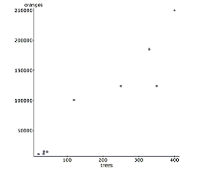 -Is the farmer in problem #5 pleased or displeased with the value of his residual? Why?
(Essay)
4.8/5 (40)
A study examined the number of trees in a variety of orange groves and the corresponding number of oranges that each
grove produces in a given harvest year. Linear regression was calculated and the results are below. linear regression results:
Dependent Variable: oranges
Independent Variable: trees
Sample size: 9
-=0.886 =31394.7
Parameter Estimate Std. Err. Constant 390.59 16328.8 Trees 525.84 71.22
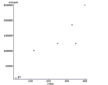 -Does the value of s concern you? How might you deal with this data differently to address
this problem?
-Does the value of s concern you? How might you deal with this data differently to address
this problem?
(Essay)
4.9/5 (37)
Taxi tires A taxi company monitoring the safety of its cabs kept track of the number of miles tires had been driven (in thousands) and the depth of the tread remaining (in mm). Their data are displayed in the scatterplot. They found the equation of the least squares regression line to be tread miles, with .
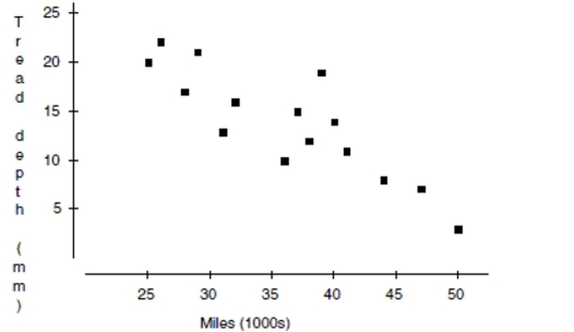 a. Draw the line of best fit on the graph. (Show your method clearly.)
b. What is the explanatory variable?
c. The correlation
d. Describe the association in context.
e. Explain (in context) what the slope of the line means.
f. Explain (in context) what the - intercept of the line means.
g. Explain (in context) what means.
h. In this context, what does a negative residual mean?
a. Draw the line of best fit on the graph. (Show your method clearly.)
b. What is the explanatory variable?
c. The correlation
d. Describe the association in context.
e. Explain (in context) what the slope of the line means.
f. Explain (in context) what the - intercept of the line means.
g. Explain (in context) what means.
h. In this context, what does a negative residual mean?
(Essay)
4.8/5 (41)
Filters
- Essay(0)
- Multiple Choice(0)
- Short Answer(0)
- True False(0)
- Matching(0)