Exam 4: Describing the Relation Between Two Variables

Compute the Sum of Squared Residuals -The regression line for the given data is $\mathrm { y } = 2.097 \mathrm { x } - 0.552$ . Determine the residual of a data point for which $x =$ $- 3$ and $y = - 8$ . -5 -3 4 1 -1 -2 0 2 3 -4 -10 -8 9 1 -2 -6 -1 3 6 -8

Compute and Interpret the Coefficient of Determination -Calculate the coefficient of determination, given that the linear correlation coefficient, r, is 1. What does this tell you about the explained variation and the unexplained variation of the data about the regression line

Compute the Sum of Squared Residuals -The data below are the ages and systolic blood pressure (measured in Millimeters of mercury) of 9 randomly selected adults. Age, Pressure, 38 116 41 12 45 123 48 131 51 142 53 145 57 148 61 150 65 152

Choose the one alternative that best completes the statement or answers the question. -The variable is the variable whose value can be explained by the variable.

Find the Least-Squares Regression Line and Use the Line to Make Predictions -A manager wishes to determine the relationship between the number of miles traveled (in hundreds of miles) by her sales representatives and their amount of sales (in thousands of dollars) per month. Find the equation of the regression line for the given data. What would be the predicted sales if the sales representative traveled 0 miles? Is this reasonable? Why or why not? Miles traveled, 2 3 10 7 8 15 3 1 11 Sales, 31 33 78 62 65 61 48 55 120

Provide an appropriate response. -The data below are the final exam scores of 10 randomly selected calculus students and the number of hours they slept the night before the exam. Calculate the linear correlation coefficient.

Write the word or phrase that best completes each statement or answers the question. Construct a scatter diagram for the data. -The data below are the temperatures on randomly chosen days during a summer class and the number of absences on those days. Temperature, x 72 85 91 90 88 98 75 100 80 Number of absences, y 3 7 10 10 8 15 4 15 5

Interpret the Slope and the y-intercept of the Least-Squares Regression Line -A large national bank charges local companies for using its services. A bank official reported the results of a regression analysis designed to predict the bank's charges (y), measured in dollars per month, for services rendered to local companies. One independent variable used to predict service charge to a company is the company's sales revenue (x), measured in millions of dollars. Data for 21 companies who use the bank's services were used to fit the model, $\hat { y } = \beta _ { 0 } + \beta _ { 1 } \mathrm { x }$ . The results of the simple linear regression are provided below. $\hat { \mathrm { y } } = 2,700 + 20 \mathrm { x } , \mathrm { s } = 65,2 \text {-tailed p-value } = 0.064 \text { (for testing } \beta _ { 1 } \text { ) }$ Interpret the estimate of $\beta _ { 0 }$ , the $y$ -intercept of the line.

Choose the one alternative that best completes the statement or answers the question. -The dean of the Business School at a small Florida college wishes to determine whether the grade-point average (GPA) of a graduating student can be used to predict the graduate's starting salary. More specifically, the dean wants to know whether higher GPA's lead to higher starting salaries. Records for 23 of last year's Business School graduates are selected at random, and data on GPA $( x )$ and starting salary ( $y$ , in Sthousands) for each graduate were used to fit the model, $\mathrm { E } ( \mathrm { y } ) = \beta _ { 0 } + \beta _ { 1 } \mathrm { x }$ . The results of the simple linear regression are provided below. =4.25+2.75, =5.15,=1.87 =15.17,=1.0075 Range of the x-values: 2.23=3.85 Range of the -values: 9.3-15.6 Range of the $\mathrm { y }$ -values: $9.3 - 15.6$ Calculate the value of $\mathrm { R } ^ { 2 }$ , the coefficient of determination.

Choose the one alternative that best completes the statement or answers the question. Use the scatter diagrams shown, labeled a through f to solve the problem. -A doctor wishes to determine the relationship between a maleʹs age and that maleʹs total cholesterol level. He tests 200 males and records each maleʹs age and that maleʹs total cholesterol level. The males cholesterol level is the predictor variable

Provide an appropriate response. -The data below are the ages and annual pharmacy b ills (in dollars) of 9 randomly selected employees. Calculate the linear correlation coefficient.

Change the exponential expression to an equivalent expression involving a logarithm. - $\log _ { b } 81 = 4$

Find the Least-Squares Regression Line and Use the Line to Make Predictions -A manager wishes to determine the relationship between the number of years her sales representatives have been employed by the firm and their amount of sales (in thousands of dollars) per month. Find the equation of the regression line for the given data. What would be the predicted sales if the sales representative was employed by the firm for 30 years Is this reasonable? Why or why not? Years employed, x 2 3 10 7 8 15 3 1 11 Sales, y 31 33 78 62 65 61 48 55 120

Provide an appropriate response. -The data below show the age and favorite type of music of 779 randomly selected people. Use $\alpha = 0.05$ . What, if any, association exists between favorite music and age? Discuss the association. Age Country Rock Pop Classical 15-21 21 45 90 33 21-30 60 55 42 48 30-40 65 47 31 57 40-50 68 39 25 53

Write the word or phrase that best completes each statement or answers the question. -Is the number of games won by a major league baseball team in a season related to the team's batting average? Data from 14 teams were collected and the summary statistics yield: $\sum \mathrm { y } = 1,134 , \sum \mathrm { x } = 3.642 , \sum \mathrm { y } ^ { 2 } = 93,110 , \sum \mathrm { x } ^ { 2 } = 0.948622 , \text { and } \sum \mathrm { xy } = 295.54$ Find the least squares prediction equation for predicting the number of games won, $y$ , using a straight-line relationship with the team's batting average, $x$ .

Interpret the Slope and the y-intercept of the Least-Squares Regression Line -Civil engineers often use the straight-line equation, $\mathrm { y } = \beta _ { 0 } + \beta _ { 1 } \mathrm { x }$ , to model the relationship between the mean shear strength of masonry joints and precompression stress, $x$ . To test this theory, a series of stress tests were performed on solid bricks arranged in triplets and joined with mortar. The precompression stress was varied for each triplet and the ultimate shear load just before failure (called the shear strength) was recorded. The stress results for $\mathrm { n } = 7$ triplet tests is shown in the accompanying table followed by a SAS printout of the regression analysis. Triplet Test 1 2 3 4 5 6 7 Shear Strength (tons), 1.00 2.18 2.24 2.41 2.59 2.82 3.06 Precomp. 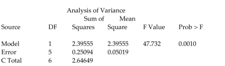Stress (tons), 0 0.60 1.20 1.33 1.43 1.75 1.75 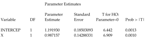Give a practical interpretation of the estimate of the slope of the least squares line.

Write the word or phrase that best completes each statement or answers the question. -Calculate the coefficient of correlation, $r$ , letting Row 1 represent the $x$ -values and Row 2 represent the $y$ -values. Now calculate the coefficient of correlation, $r$ , letting Row 2 represent the $x$ -values and Row 1 represent the $y$ -values. What effect does switching the explanatory and response variables have on the linear correlation coefficient?

Compute and Interpret the Coefficient of Determination -Calculate the coefficient of determination, given that the linear correlation coefficient, r, is 0.837. What does this tell you about the explained variation and the unexplained variation of the data about the regression line

Choose the one alternative that best completes the statement or answers the question. -In an area of Russia, records were kept on the relationship between the rainfall (in inches) and the yield of wheat (bushels per acre). The data for a 9 year period is as follows: Rain Fall, x 13.1 11.4 16.0 15.1 21.4 12.9 9.6 18.2 18.6 Yield, y 48.5 44.2 56.8 80.4 47.2 29.9 74.0 74.0 76.8 The equation of the line of least squares is given as $\mathrm { y } = - 9.12 + 4.38 \mathrm { x }$ . How many bushels of wheat per acre can be predicted if it is expected that there will be 30 inches of rain?

Perform Residual Analysis on a Regression Model -