Exam 18: A Roadmap for Analyzing Data

SCENARIO 18-9 What are the factors that determine the acceleration time (in sec.)from 0 to 60 miles per hour of a car? Data on the following variables for 171 different vehicle models were collected: Accel Time: Acceleration time in sec. Cargo Vol: Cargo volume in cu.ft. HP: Horsepower MPG: Miles per gallon SUV: 1 if the vehicle model is an SUV with Coupe as the base when SUV and Sedan are both 0 Sedan: 1 if the vehicle model is a sedan with Coupe as the base when SUV and Sedan are both 0 The regression results using acceleration time as the dependent variable and the remaining variables as the independent variables are presented below. SCENARIO 18-9 cont. 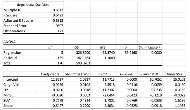The various residual plots are as shown below. 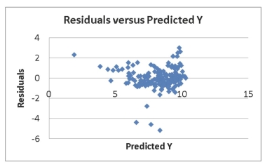SCENARIO 18-9 cont. 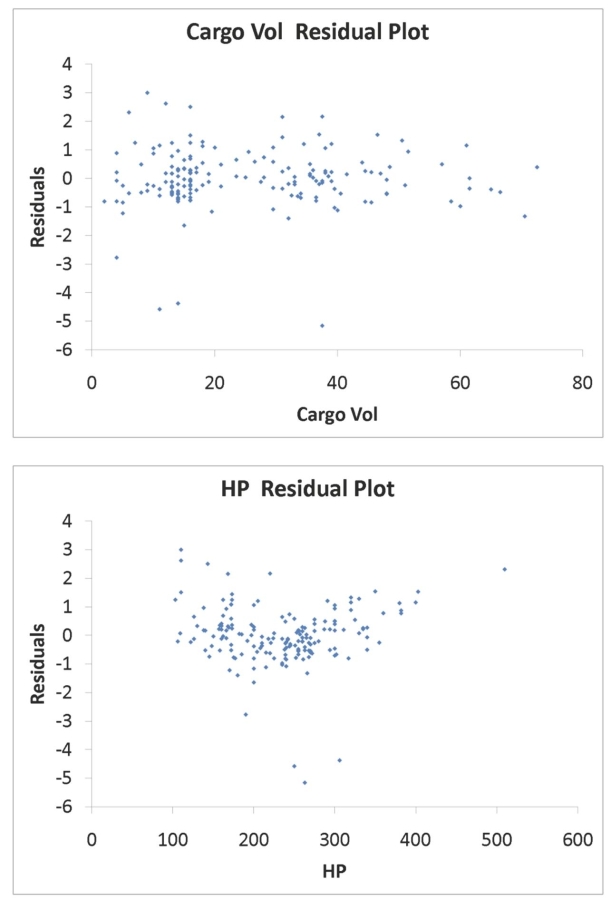SCENARIO 18-9 cont. 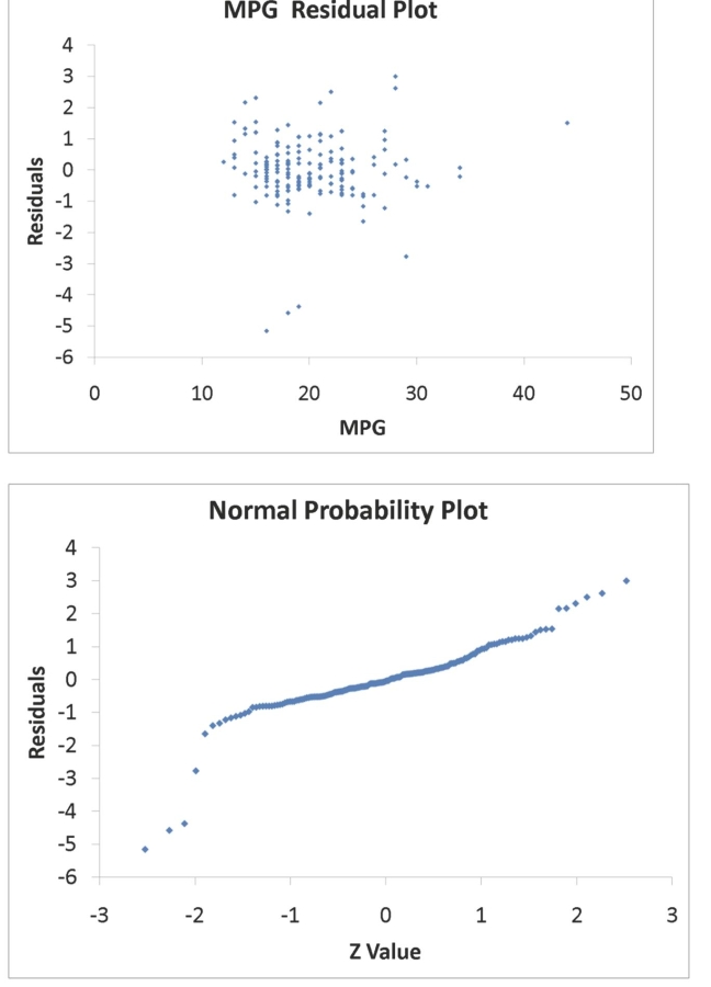The coefficient of partial determination 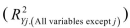of each of the 5 predictors are, respectively, 0.0380, 0.4376, 0.0248, 0.0188, and 0.0312. The coefficient of multiple determination for the regression model using each of the 5 variables as the dependent variable and all other X variables as independent variables ( )are, respectively, 0.7461, 0.5676, 0.6764, 0.8582, 0.6632. -Referring to Scenario 18-9, what is the value of the test statistic to determine whether HP makes a significant contribution to the regression model in the presence of the other independent variables at a 5% level of significance?

SCENARIO 18-11 A logistic regression model was estimated in order to predict the probability that a randomly chosen university or college would be a private university using information on mean total Scholastic Aptitude Test score (SAT)at the university or college, the room and board expense measured in thousands of dollars (Room/Brd), and whether the TOEFL criterion is at least 550 (Toefl550 = 1 if yes, 0 otherwise.)The dependent variable, Y, is school type (Type = 1 if private and 0 otherwise). The Minitab output is given below: 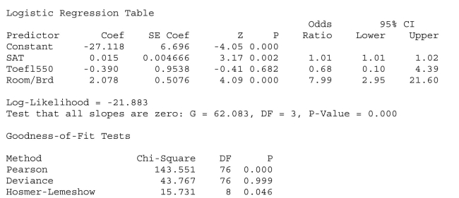-Referring to Scenario 18-11, there is not enough evidence to conclude that Toefl500 makes a significant contribution to the model in the presence of the other independent variables at a 0.05 level of significance.

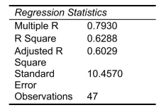
SCENARIO 18-4 You decide to predict gasoline prices in different cities and towns in the United States for your term project.Your dependent variable is price of gasoline per gallon and your explanatory variables are per capita income, the number of firms that manufacture automobile parts in and around the city, the number of new business starts in the last year, population density of the city, percentage of local taxes on gasoline, and the number of people using public transportation.You collected data of 32 cities and obtained a regression sum of squares SSR= 122.8821.Your computed value of standard error of the estimate is 1.9549. -Referring to Scenario 18-4, if variables that measure the number of new business starts in the last year and population density of the city were removed from the multiple regression model, which of the following would be true?

A pizza chain is considering opening a new store in an area that currently does not have any such stores.The chain will open if there is evidence that more than 5,000 of the 20,000 households in the area have a favorable view of its brand.It conducts a telephone poll of 300 randomly selected households in the area and finds that 96 have a favorable view. Which of the following tests will be the most appropriate?

SCENARIO 18-8 The superintendent of a school district wanted to predict the percentage of students passing a sixth-grade proficiency test.She obtained the data on percentage of students passing the proficiency test (% Passing), daily mean of the percentage of students attending class (% Attendance), mean teacher salary in dollars (Salaries), and instructional spending per pupil in dollars (Spending)of 47 schools in the state. Following is the multiple regression output with as the dependent variable, -Referring to Scenario 18-8, the alternative hypothesis : At least one of for j = 1, 2, 3 implies that percentage of students passing the proficiency test is affected by all of the explanatory variables.

SCENARIO 18-11 A logistic regression model was estimated in order to predict the probability that a randomly chosen university or college would be a private university using information on mean total Scholastic Aptitude Test score (SAT)at the university or college, the room and board expense measured in thousands of dollars (Room/Brd), and whether the TOEFL criterion is at least 550 (Toefl550 = 1 if yes, 0 otherwise.)The dependent variable, Y, is school type (Type = 1 if private and 0 otherwise). The Minitab output is given below: -Referring to Scenario 18-11, what should be the decision ('reject' or 'do not reject')on the null hypothesis when testing whether Toefl500 makes a significant contribution to the model in the presence of the other independent variables at a 0.05 level of significance?

An entrepreneur is considering the purchase of a coin-operated laundry.The current owner claims that over the past 5 years, the mean daily revenue was $675 with a standard deviation of $75.A sample of 30 days reveals a daily mean revenue of $625 and a standard deviation of $70.Which of the following tests will be the most appropriate?

SCENARIO 18-12 The marketing manager for a nationally franchised lawn service company would like to study the characteristics that differentiate home owners who do and do not have a lawn service.A random sample of 30 home owners located in a suburban area near a large city was selected; 15 did not have a lawn service (code 0)and 15 had a lawn service (code 1).Additional information available concerning these 30 home owners includes family income (Income, in thousands of dollars), lawn size (Lawn Size, in thousands of square feet), attitude toward outdoor recreational activities (Attitude 0 = unfavorable, 1 = favorable), number of teenagers in the household (Teenager), and age of the head of the household (Age). The Minitab output is given below: 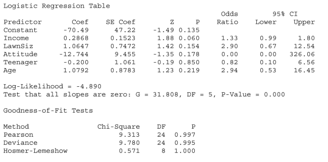-Referring to Scenario 18-12, there is not enough evidence to conclude that Income makes a significant contribution to the model in the presence of the other independent variables at a 0.05 level of significance.

SCENARIO 18-7 As a project for his business statistics class, a student examined the factors that determined parking meter rates throughout the campus area.Data were collected for the price per hour of parking, blocks to the quadrangle, and one of the three jurisdictions: on campus, in downtown and off campus, or outside of downtown and off campus.The population regression model hypothesized is where Y is the meter price is the number of blocks to the quad is a dummy variable that takes the value 1 if the meter is located in downtown and off campus and the value 0 otherwise is a dummy variable that takes the value 1 if the meter is located outside of downtown and off campus, and the value 0 otherwise The following Excel results are obtained. 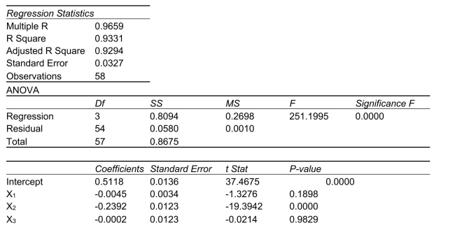-Referring to Scenario 18-7, what is the correct interpretation for the estimated coefficient for

SCENARIO 18-1 A real estate builder wishes to determine how house size (House)is influenced by family income (Income), family size (Size), and education of the head of household (School).House size is measured in hundreds of square feet, income is measured in thousands of dollars, and education is in years.The builder randomly selected 50 families and ran the multiple regression.Microsoft Excel output is provided below: SUMMARY OUTPUT 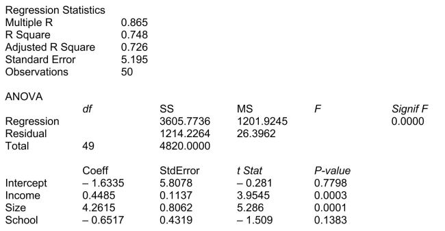-Referring to Scenario 18-1, what minimum annual income would an individual with a family size of 9 and 10 years of education need to attain a predicted 5,000 square foot home (House = 50)?

SCENARIO 18-11 A logistic regression model was estimated in order to predict the probability that a randomly chosen university or college would be a private university using information on mean total Scholastic Aptitude Test score (SAT)at the university or college, the room and board expense measured in thousands of dollars (Room/Brd), and whether the TOEFL criterion is at least 550 (Toefl550 = 1 if yes, 0 otherwise.)The dependent variable, Y, is school type (Type = 1 if private and 0 otherwise). The Minitab output is given below: -Referring to Scenario 18-11, what is the estimated probability that a school with a mean SAT score of 1100, a TOEFL criterion that is not at least 550, and the room and board expense of 7 thousand dollars will be a private school?

SCENARIO 18-10 Given below are results from the regression analysis where the dependent variable is the number of weeks a worker is unemployed due to a layoff (Unemploy)and the independent variables are the age of the worker (Age), the number of years of education received (Edu), the number of years at the previous job (Job Yr), a dummy variable for marital status (Married: 1 = married, 0 = otherwise), a dummy variable for head of household (Head: 1 = yes, 0 = no)and a dummy variable for management position (Manager: 1 = yes, 0 = no).We shall call this Model 1.The coefficient of partial determination 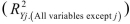of each of the 6 predictors are, respectively, 0.2807, 0.0386, 0.0317, 0.0141, 0.0958, and 0.1201. 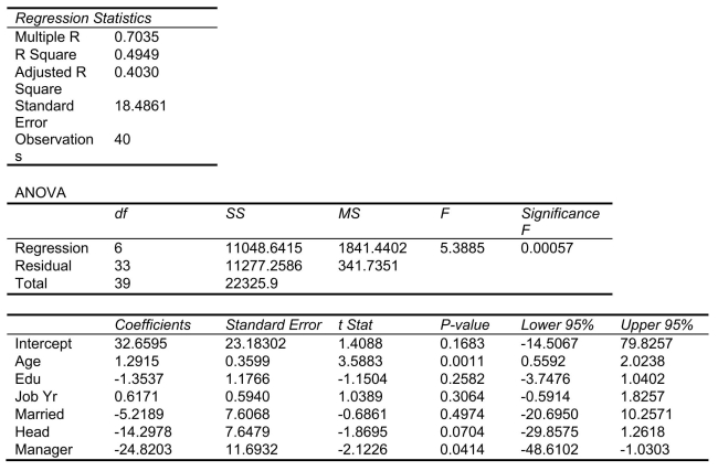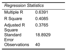Model 2 is the regression analysis where the dependent variable is Unemploy and the independent variables are Age and Manager.The results of the regression analysis are given below: 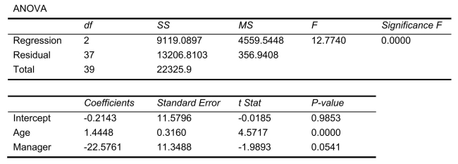-Referring to Scenario 18-10 and using both Model 1 and Model 2, what is the critical value of the test statistic for testing whether the independent variables that are not significant individually are also not significant as a group in explaining the variation in the dependent variable at a 5% level of significance?

SCENARIO 18-12 The marketing manager for a nationally franchised lawn service company would like to study the characteristics that differentiate home owners who do and do not have a lawn service.A random sample of 30 home owners located in a suburban area near a large city was selected; 15 did not have a lawn service (code 0)and 15 had a lawn service (code 1).Additional information available concerning these 30 home owners includes family income (Income, in thousands of dollars), lawn size (Lawn Size, in thousands of square feet), attitude toward outdoor recreational activities (Attitude 0 = unfavorable, 1 = favorable), number of teenagers in the household (Teenager), and age of the head of the household (Age). The Minitab output is given below: -Referring to Scenario 18-12, what should be the decision ('reject' or 'do not reject')on the null hypothesis when testing whether LawnSize makes a significant contribution to the model in the presence of the other independent variables at a 0.05 level of significance?

SCENARIO 18-2 One of the most common questions of prospective house buyers pertains to the cost of heating in dollars (Y).To provide its customers with information on that matter, a large real estate firm used the following 4 variables to predict heating costs: the daily minimum outside temperature in degrees of Fahrenheit ( ), the amount of insulation in inches ( ), the number of windows in the house ( ), and the age of the furnace in years ( ).Given below are the EXCEL outputs of two regression models. 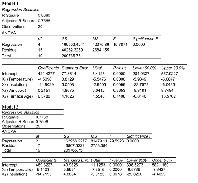-Referring to Scenario 18-2 and allowing for a 1% probability of committing a type I error, what is the decision and conclusion for the test j =1, 2,..., 4 using Model 1?

SCENARIO 18-10 Given below are results from the regression analysis where the dependent variable is the number of weeks a worker is unemployed due to a layoff (Unemploy)and the independent variables are the age of the worker (Age), the number of years of education received (Edu), the number of years at the previous job (Job Yr), a dummy variable for marital status (Married: 1 = married, 0 = otherwise), a dummy variable for head of household (Head: 1 = yes, 0 = no)and a dummy variable for management position (Manager: 1 = yes, 0 = no).We shall call this Model 1.The coefficient of partial determination of each of the 6 predictors are, respectively, 0.2807, 0.0386, 0.0317, 0.0141, 0.0958, and 0.1201. Model 2 is the regression analysis where the dependent variable is Unemploy and the independent variables are Age and Manager.The results of the regression analysis are given below: -Referring to Scenario 18-10 Model 1, what are the numerator and denominator degrees of freedom, respectively, for the test statistic to determine whether there is a significant relationship between the number of weeks a worker is unemployed due to a layoff and the entire set of explanatory variables?

SCENARIO 18-9 What are the factors that determine the acceleration time (in sec.)from 0 to 60 miles per hour of a car? Data on the following variables for 171 different vehicle models were collected: Accel Time: Acceleration time in sec. Cargo Vol: Cargo volume in cu.ft. HP: Horsepower MPG: Miles per gallon SUV: 1 if the vehicle model is an SUV with Coupe as the base when SUV and Sedan are both 0 Sedan: 1 if the vehicle model is a sedan with Coupe as the base when SUV and Sedan are both 0 The regression results using acceleration time as the dependent variable and the remaining variables as the independent variables are presented below. SCENARIO 18-9 cont. The various residual plots are as shown below. SCENARIO 18-9 cont. SCENARIO 18-9 cont. The coefficient of partial determination of each of the 5 predictors are, respectively, 0.0380, 0.4376, 0.0248, 0.0188, and 0.0312. The coefficient of multiple determination for the regression model using each of the 5 variables as the dependent variable and all other X variables as independent variables ( )are, respectively, 0.7461, 0.5676, 0.6764, 0.8582, 0.6632. -Referring to Scenario 18-9, what is the p-value of the test statistic to determine whether HP makes a significant contribution to the regression model in the presence of the other independent variables at a 5% level of significance?

The owner of a local nightclub has recently surveyed a random sample of n = 250 customers of the club.She would now like to determine whether or not the mean age of her customers is more than 30.If so, she plans to alter the entertainment to appeal to an older crowd.If not, no entertainment changes will be made.Which of the following tests will you perform to help her decide?

SCENARIO 18-1 A real estate builder wishes to determine how house size (House)is influenced by family income (Income), family size (Size), and education of the head of household (School).House size is measured in hundreds of square feet, income is measured in thousands of dollars, and education is in years.The builder randomly selected 50 families and ran the multiple regression.Microsoft Excel output is provided below: SUMMARY OUTPUT -Referring to Scenario 18-1, one individual in the sample had an annual income of $40,000, a family size of 1, and an education of 8 years.This individual owned a home with an area of 1,000 square feet (House = 10.00).What is the residual (in hundreds of square feet)for this data point?

SCENARIO 18-12 The marketing manager for a nationally franchised lawn service company would like to study the characteristics that differentiate home owners who do and do not have a lawn service.A random sample of 30 home owners located in a suburban area near a large city was selected; 15 did not have a lawn service (code 0)and 15 had a lawn service (code 1).Additional information available concerning these 30 home owners includes family income (Income, in thousands of dollars), lawn size (Lawn Size, in thousands of square feet), attitude toward outdoor recreational activities (Attitude 0 = unfavorable, 1 = favorable), number of teenagers in the household (Teenager), and age of the head of the household (Age). The Minitab output is given below: -Referring to Scenario 18-12, what is the p-value of the test statistic when testing whether Age makes a significant contribution to the model in the presence of the other independent variables?

SCENARIO 18-6 A weight-loss clinic wants to use regression analysis to build a model for weight-loss of a client (measured in pounds).Two variables thought to affect weight-loss are client's length of time on the weight loss program and time of session.These variables are described below: Y = Weight-loss (in pounds) = Length of time in weight-loss program (in months) = 1 if morning session, 0 if not = 1 if afternoon session, 0 if not (Base level = evening session) Data for 12 clients on a weight-loss program at the clinic were collected and used to fit the interaction model: Partial output from Microsoft Excel follows: 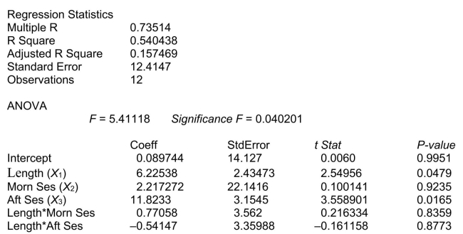-Referring to Scenario 18-6, in terms of the in the model, give the mean change in weight-loss (Y)for every 1 month increase in time in the program ( when attending the afternoon session.