Exam 18: A Roadmap for Analyzing Data

Suppose that past history shows that 6% of college students prefer Brand A Cola.A sample of 10,000 students is to be selected.Which of the following distributions would you use to compute the probability that at least half of them will prefer Brand A cola?

SCENARIO 18-10 Given below are results from the regression analysis where the dependent variable is the number of weeks a worker is unemployed due to a layoff (Unemploy)and the independent variables are the age of the worker (Age), the number of years of education received (Edu), the number of years at the previous job (Job Yr), a dummy variable for marital status (Married: 1 = married, 0 = otherwise), a dummy variable for head of household (Head: 1 = yes, 0 = no)and a dummy variable for management position (Manager: 1 = yes, 0 = no).We shall call this Model 1.The coefficient of partial determination 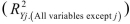of each of the 6 predictors are, respectively, 0.2807, 0.0386, 0.0317, 0.0141, 0.0958, and 0.1201. 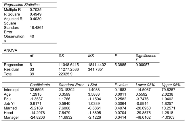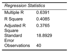Model 2 is the regression analysis where the dependent variable is Unemploy and the independent variables are Age and Manager.The results of the regression analysis are given below: -Referring to Scenario 18-10 Model 1, what is the value of the test statistic when testing whether being married or not makes a difference in the mean number of weeks a worker is unemployed due to a layoff while holding constant the effect of all the other independent variables?

SCENARIO 18-6 A weight-loss clinic wants to use regression analysis to build a model for weight-loss of a client (measured in pounds).Two variables thought to affect weight-loss are client's length of time on the weight loss program and time of session.These variables are described below: Y = Weight-loss (in pounds) = Length of time in weight-loss program (in months) = 1 if morning session, 0 if not = 1 if afternoon session, 0 if not (Base level = evening session) Data for 12 clients on a weight-loss program at the clinic were collected and used to fit the interaction model: Partial output from Microsoft Excel follows: 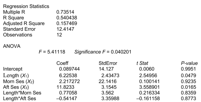-Referring to Scenario 18-6, the overall model for predicting weight-loss (Y) is statistically significant at the 0.05 level.

A buyer for a manufacturing plant suspects that his primary supplier of raw materials is overcharging.In order to determine if his suspicion is correct, he contacts a second supplier and asks for the prices on various identical materials.He wants to compare these prices with those of his primary supplier.He collected data on 6 different materials from both suppliers.He believes that the differences are normally distributed.Which of the following tests will be the most appropriate?

SCENARIO 18-10 Given below are results from the regression analysis where the dependent variable is the number of weeks a worker is unemployed due to a layoff (Unemploy)and the independent variables are the age of the worker (Age), the number of years of education received (Edu), the number of years at the previous job (Job Yr), a dummy variable for marital status (Married: 1 = married, 0 = otherwise), a dummy variable for head of household (Head: 1 = yes, 0 = no)and a dummy variable for management position (Manager: 1 = yes, 0 = no).We shall call this Model 1.The coefficient of partial determination of each of the 6 predictors are, respectively, 0.2807, 0.0386, 0.0317, 0.0141, 0.0958, and 0.1201. Model 2 is the regression analysis where the dependent variable is Unemploy and the independent variables are Age and Manager.The results of the regression analysis are given below: -Referring to Scenario 18-10 Model 1, ________ of the variation in the number of weeks a worker is unemployed due to a layoff can be explained by the number of years at the previous job while controlling for the other independent variables.

SCENARIO 18-11 A logistic regression model was estimated in order to predict the probability that a randomly chosen university or college would be a private university using information on mean total Scholastic Aptitude Test score (SAT)at the university or college, the room and board expense measured in thousands of dollars (Room/Brd), and whether the TOEFL criterion is at least 550 (Toefl550 = 1 if yes, 0 otherwise.)The dependent variable, Y, is school type (Type = 1 if private and 0 otherwise). The Minitab output is given below: 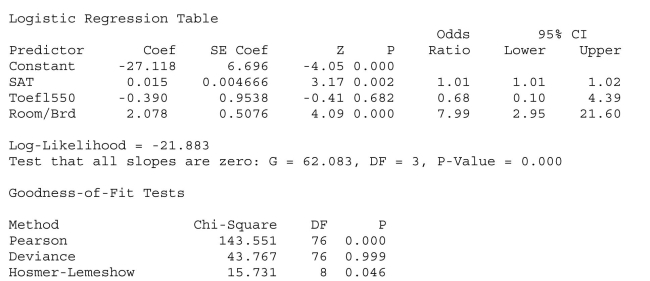-Referring to Scenario 18-11, which of the following is the correct interpretation for the SAT slope coefficient?

SCENARIO 18-10 Given below are results from the regression analysis where the dependent variable is the number of weeks a worker is unemployed due to a layoff (Unemploy)and the independent variables are the age of the worker (Age), the number of years of education received (Edu), the number of years at the previous job (Job Yr), a dummy variable for marital status (Married: 1 = married, 0 = otherwise), a dummy variable for head of household (Head: 1 = yes, 0 = no)and a dummy variable for management position (Manager: 1 = yes, 0 = no).We shall call this Model 1.The coefficient of partial determination of each of the 6 predictors are, respectively, 0.2807, 0.0386, 0.0317, 0.0141, 0.0958, and 0.1201. Model 2 is the regression analysis where the dependent variable is Unemploy and the independent variables are Age and Manager.The results of the regression analysis are given below: -Referring to Scenario 18-10 Model 1, ________ of the variation in the number of weeks a worker is unemployed due to a layoff can be explained by the six independent variables after taking into consideration the number of independent variables and the number of observations.

SCENARIO 18-5 You worked as an intern at We Always Win Car Insurance Company last summer.You notice that individual car insurance premiums depend very much on the age of the individual, the number of traffic tickets received by the individual, and the population density of the city in which the individual lives.You performed a regression analysis in EXCEL and obtained the following information: Regression Analysis 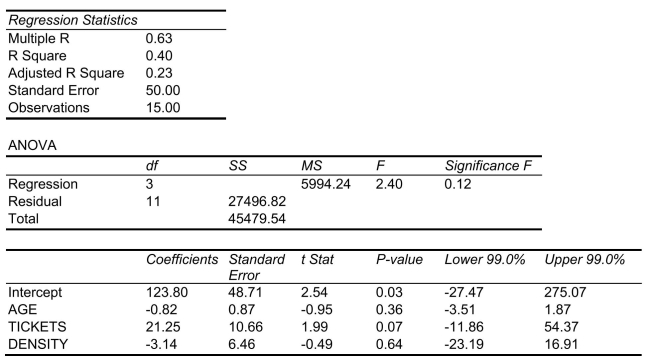-Referring to Scenario 18-5, the residual mean squares (MSE)that are missing in the ANOVA table should be _____.

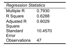
SCENARIO 18-8 The superintendent of a school district wanted to predict the percentage of students passing a sixth-grade proficiency test.She obtained the data on percentage of students passing the proficiency test (% Passing), daily mean of the percentage of students attending class (% Attendance), mean teacher salary in dollars (Salaries), and instructional spending per pupil in dollars (Spending)of 47 schools in the state. Following is the multiple regression output with as the dependent variable, -Referring to Scenario 18-8, which of the following is the correct alternative hypothesis to test whether daily mean of the percentage of students attending class has any effect on percentage of students passing the proficiency test, considering the effect of all the other independent variables?

Suppose the probability of finding a defective spot in an area on a piece of glass is the ratio of that area to the total area of the glass and the probability is the same across the whole glass.Which of the following distributions would you use to determine the probability of finding a defective spot in a randomly selected one square inch area on a piece of 10 feet by 10 feet glass?

SCENARIO 18-9 What are the factors that determine the acceleration time (in sec.)from 0 to 60 miles per hour of a car? Data on the following variables for 171 different vehicle models were collected: Accel Time: Acceleration time in sec. Cargo Vol: Cargo volume in cu.ft. HP: Horsepower MPG: Miles per gallon SUV: 1 if the vehicle model is an SUV with Coupe as the base when SUV and Sedan are both 0 Sedan: 1 if the vehicle model is a sedan with Coupe as the base when SUV and Sedan are both 0 The regression results using acceleration time as the dependent variable and the remaining variables as the independent variables are presented below. SCENARIO 18-9 cont. 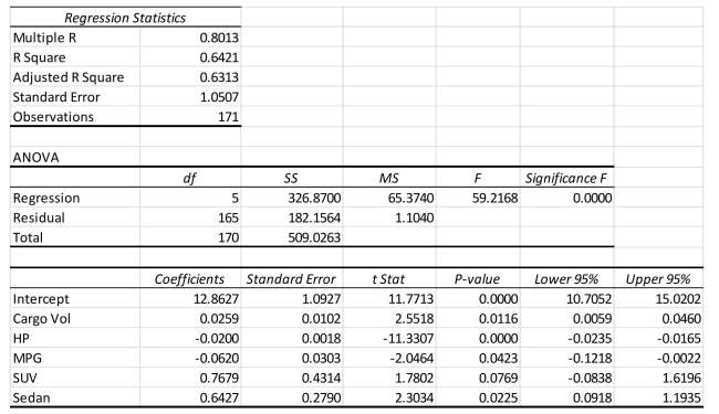The various residual plots are as shown below. 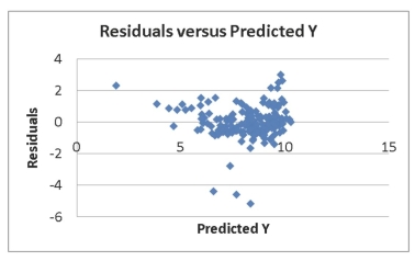SCENARIO 18-9 cont. 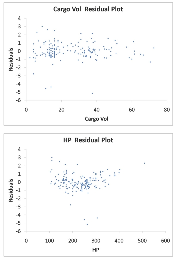SCENARIO 18-9 cont. 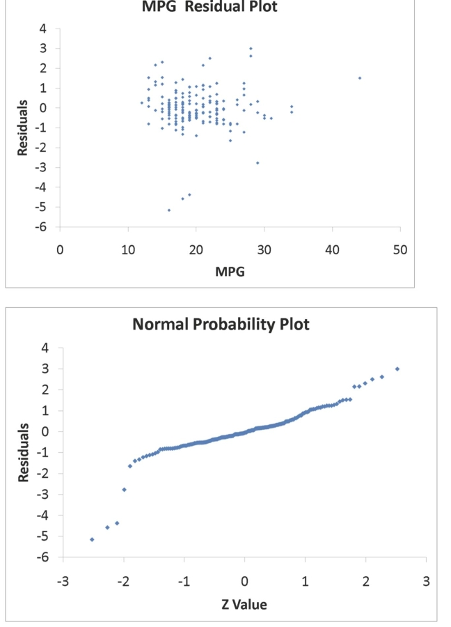The coefficient of partial determination 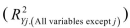of each of the 5 predictors are, respectively, 0.0380, 0.4376, 0.0248, 0.0188, and 0.0312. The coefficient of multiple determination for the regression model using each of the 5 variables as the dependent variable and all other X variables as independent variables ( )are, respectively, 0.7461, 0.5676, 0.6764, 0.8582, 0.6632. -Referring to Scenario 18-9, there is enough evidence to conclude that SUV makes a significant contribution to the regression model in the presence of the other independent variables at a 5% level of significance.

SCENARIO 18-8 The superintendent of a school district wanted to predict the percentage of students passing a sixth-grade proficiency test.She obtained the data on percentage of students passing the proficiency test (% Passing), daily mean of the percentage of students attending class (% Attendance), mean teacher salary in dollars (Salaries), and instructional spending per pupil in dollars (Spending)of 47 schools in the state. Following is the multiple regression output with as the dependent variable, -Referring to Scenario 18-8, there is sufficient evidence that instructional spending per pupil has an effect on percentage of students passing the proficiency test while holding constant the effect of all the other independent variables at a 5% level of significance.

SCENARIO 18-10 Given below are results from the regression analysis where the dependent variable is the number of weeks a worker is unemployed due to a layoff (Unemploy)and the independent variables are the age of the worker (Age), the number of years of education received (Edu), the number of years at the previous job (Job Yr), a dummy variable for marital status (Married: 1 = married, 0 = otherwise), a dummy variable for head of household (Head: 1 = yes, 0 = no)and a dummy variable for management position (Manager: 1 = yes, 0 = no).We shall call this Model 1.The coefficient of partial determination of each of the 6 predictors are, respectively, 0.2807, 0.0386, 0.0317, 0.0141, 0.0958, and 0.1201. Model 2 is the regression analysis where the dependent variable is Unemploy and the independent variables are Age and Manager.The results of the regression analysis are given below: -Referring to Scenario 18-10 Model 1, we can conclude that, holding constant the effect of the other independent variables, the number of years of education received has no impact on the mean number of weeks a worker is unemployed due to a layoff at a 1% level of significance if all we have is the information of the 95% confidence interval estimate for .

SCENARIO 18-8 The superintendent of a school district wanted to predict the percentage of students passing a sixth-grade proficiency test.She obtained the data on percentage of students passing the proficiency test (% Passing), daily mean of the percentage of students attending class (% Attendance), mean teacher salary in dollars (Salaries), and instructional spending per pupil in dollars (Spending)of 47 schools in the state. Following is the multiple regression output with as the dependent variable, -Referring to Scenario 18-8, the null hypothesis 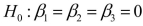implies that percentage of students passing the proficiency test is not related to any of the explanatory variables.

A certain type of rare gem serves as a status symbol for many of its owners.In theory, for low prices, the demand increases, and it decreases as the price of the gem increases. However, experts hypothesize that when the gem is valued at very high prices, the demand increases with price due to the status owners believe they gain in obtaining the gem.Data on price and quantity sold were collected for a sample of 35 rare gems of this type.Which of the following would be the most appropriate analysis to perform?

SCENARIO 18-2 One of the most common questions of prospective house buyers pertains to the cost of heating in dollars (Y).To provide its customers with information on that matter, a large real estate firm used the following 4 variables to predict heating costs: the daily minimum outside temperature in degrees of Fahrenheit ( ), the amount of insulation in inches ( ), the number of windows in the house ( ), and the age of the furnace in years ( ).Given below are the EXCEL outputs of two regression models. 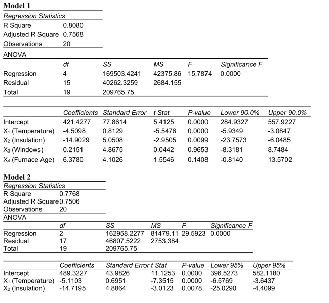-Referring to Scenario 18-2, what is the value of the partial F test statistic for j =3, 4 ?

An agronomist wants to compare the crop yield of 3 varieties of chickpea seeds.She plants all 3 varieties of the seeds on each of 5 different patches of fields.She then measures the crop yield in bushels per acre.She has found out that the different varieties do have an impact on crop yield.Which of the following tests will be the most appropriate to find out which variety will produce the highest yield?

Suppose students arrive at an advising office at a rate of 30 per hour.Which of the following distributions would you use to determine the probability that the next two students will arrive 30 minutes apart?

A survey claims that 9 out of 10 doctors recommend aspirin for their patients with headaches.To test this claim, a random sample of 100 doctors results in 83 who indicate that they recommend aspirin.Which of the following tests will you perform?

SCENARIO 18-8 The superintendent of a school district wanted to predict the percentage of students passing a sixth-grade proficiency test.She obtained the data on percentage of students passing the proficiency test (% Passing), daily mean of the percentage of students attending class (% Attendance), mean teacher salary in dollars (Salaries), and instructional spending per pupil in dollars (Spending)of 47 schools in the state. Following is the multiple regression output with as the dependent variable, -Referring to Scenario 18-8, which of the following is the correct alternative hypothesis to test whether instructional spending per pupil has any effect on percentage of students passing the proficiency test, considering the effect of all the other independent variables?