Exam 18: A Roadmap for Analyzing Data

SCENARIO 18-10 Given below are results from the regression analysis where the dependent variable is the number of weeks a worker is unemployed due to a layoff (Unemploy)and the independent variables are the age of the worker (Age), the number of years of education received (Edu), the number of years at the previous job (Job Yr), a dummy variable for marital status (Married: 1 = married, 0 = otherwise), a dummy variable for head of household (Head: 1 = yes, 0 = no)and a dummy variable for management position (Manager: 1 = yes, 0 = no).We shall call this Model 1.The coefficient of partial determination of each of the 6 predictors are, respectively, 0.2807, 0.0386, 0.0317, 0.0141, 0.0958, and 0.1201. 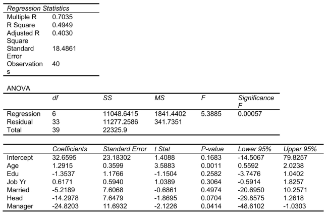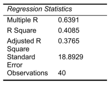Model 2 is the regression analysis where the dependent variable is Unemploy and the independent variables are Age and Manager.The results of the regression analysis are given below: -Referring to Scenario 18-10 Model 1, there is sufficient evidence that the number of weeks a worker is unemployed due to a layoff depends on all of the explanatory variables at a 10% level of significance.

A few years ago, Pepsi invited consumers to take the "Pepsi Challenge." Consumers were asked to decide which of two sodas, Coke or Pepsi, they preferred in a blind taste test. Pepsi was interesting in determining what factors played a role in people's taste preferences.One of the factors studied was the gender of the consumer.Data on the percentage of men and women depicting preference for Pepsi were collected.Which of the following tests will you use to find out if there is any difference in preference between the different gender groups?

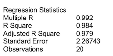
SCENARIO 18-3 A financial analyst wanted to examine the relationship between salary (in $1,000)and 4 variables: age ( = Age), experience in the field ( = Exper), number of degrees ( = Degrees), and number of previous jobs in the field ( = Prevjobs).He took a sample of 20 employees and obtained the following Microsoft Excel output: SUMMARY OUTPUT -Referring to Scenario 18-3, the critical value of an F test on the entire regression for a level of significance of 0.01 is ________.

SCENARIO 18-10 Given below are results from the regression analysis where the dependent variable is the number of weeks a worker is unemployed due to a layoff (Unemploy)and the independent variables are the age of the worker (Age), the number of years of education received (Edu), the number of years at the previous job (Job Yr), a dummy variable for marital status (Married: 1 = married, 0 = otherwise), a dummy variable for head of household (Head: 1 = yes, 0 = no)and a dummy variable for management position (Manager: 1 = yes, 0 = no).We shall call this Model 1.The coefficient of partial determination of each of the 6 predictors are, respectively, 0.2807, 0.0386, 0.0317, 0.0141, 0.0958, and 0.1201. Model 2 is the regression analysis where the dependent variable is Unemploy and the independent variables are Age and Manager.The results of the regression analysis are given below: -Referring to Scenario 18-10 Model 1, ________ of the variation in the number of weeks a worker is unemployed due to a layoff can be explained by the marital status while controlling for the other independent variables.

SCENARIO 18-3 A financial analyst wanted to examine the relationship between salary (in $1,000)and 4 variables: age ( = Age), experience in the field ( = Exper), number of degrees ( = Degrees), and number of previous jobs in the field ( = Prevjobs).He took a sample of 20 employees and obtained the following Microsoft Excel output: SUMMARY OUTPUT -Referring to Scenario 18-3, the F test for the significance of the entire regression performed at a level of significance of 0.01 leads to a rejection of the null hypothesis.

SCENARIO 18-10 Given below are results from the regression analysis where the dependent variable is the number of weeks a worker is unemployed due to a layoff (Unemploy)and the independent variables are the age of the worker (Age), the number of years of education received (Edu), the number of years at the previous job (Job Yr), a dummy variable for marital status (Married: 1 = married, 0 = otherwise), a dummy variable for head of household (Head: 1 = yes, 0 = no)and a dummy variable for management position (Manager: 1 = yes, 0 = no).We shall call this Model 1.The coefficient of partial determination of each of the 6 predictors are, respectively, 0.2807, 0.0386, 0.0317, 0.0141, 0.0958, and 0.1201. Model 2 is the regression analysis where the dependent variable is Unemploy and the independent variables are Age and Manager.The results of the regression analysis are given below: -Referring to Scenario 18-10 Model 1, which of the following is the correct alternative hypothesis to test whether age has any effect on the number of weeks a worker is unemployed due to a layoff while holding constant the effect of all the other independent variables?

An airline wants to select a computer software package for its reservation system.Four software packages (1, 2, 3, and 4)are commercially available.An experiment is set up in which each package is used to make reservations for 5 randomly selected weeks and data on the number of passengers that are bumped over a month are collected.(A total of 20 weeks was included in the experiment.)The variance on the number of passengers that are bumped is found to be roughly the same for the 4 packages.Which of the following tests will be the most appropriate to find out if the mean number of passengers being bumped over a month is the same across the 4 packages?

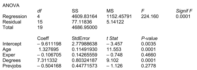
SCENARIO 18-5 You worked as an intern at We Always Win Car Insurance Company last summer.You notice that individual car insurance premiums depend very much on the age of the individual, the number of traffic tickets received by the individual, and the population density of the city in which the individual lives.You performed a regression analysis in EXCEL and obtained the following information: Regression Analysis -Referring to Scenario 18-5, to test the significance of the multiple regression model, what is the form of the null hypothesis?

SCENARIO 18-1 A real estate builder wishes to determine how house size (House)is influenced by family income (Income), family size (Size), and education of the head of household (School).House size is measured in hundreds of square feet, income is measured in thousands of dollars, and education is in years.The builder randomly selected 50 families and ran the multiple regression.Microsoft Excel output is provided below: SUMMARY OUTPUT 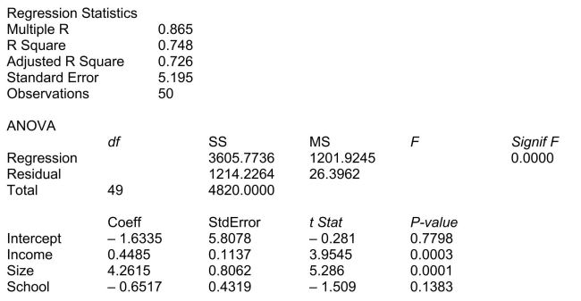-Referring to Scenario 18-1, one individual in the sample had an annual income of $100,000, a family size of 10, and an education of 16 years.This individual owned a home with an area of 7,000 square feet (House = 70.00).What is the residual (in hundreds of square feet)for this data point?

The opinions (classified as "for", "neutral" or "against")of a sample of 200 people broken down by gender about the latest congressional plan to eliminate anti-trust exemptions for professional baseball.You can present this information using a scatter plot.

SCENARIO 18-10 Given below are results from the regression analysis where the dependent variable is the number of weeks a worker is unemployed due to a layoff (Unemploy)and the independent variables are the age of the worker (Age), the number of years of education received (Edu), the number of years at the previous job (Job Yr), a dummy variable for marital status (Married: 1 = married, 0 = otherwise), a dummy variable for head of household (Head: 1 = yes, 0 = no)and a dummy variable for management position (Manager: 1 = yes, 0 = no).We shall call this Model 1.The coefficient of partial determination of each of the 6 predictors are, respectively, 0.2807, 0.0386, 0.0317, 0.0141, 0.0958, and 0.1201. Model 2 is the regression analysis where the dependent variable is Unemploy and the independent variables are Age and Manager.The results of the regression analysis are given below: -Referring to Scenario 18-10 Model 1, ________ of the variation in the number of weeks a worker is unemployed due to a layoff can be explained by the number of years of education received while controlling for the other independent variables.

SCENARIO 18-8 The superintendent of a school district wanted to predict the percentage of students passing a sixth-grade proficiency test.She obtained the data on percentage of students passing the proficiency test (% Passing), daily mean of the percentage of students attending class (% Attendance), mean teacher salary in dollars (Salaries), and instructional spending per pupil in dollars (Spending)of 47 schools in the state. 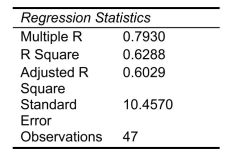Following is the multiple regression output with as the dependent variable, -Referring to Scenario 18-8, you can conclude that average teacher salary individually has no impact on the mean percentage of students passing the proficiency test, considering the effect of all the other independent variables, at a 10% level of significance based solely on the 95% confidence interval estimate for .

SCENARIO 18-10 Given below are results from the regression analysis where the dependent variable is the number of weeks a worker is unemployed due to a layoff (Unemploy)and the independent variables are the age of the worker (Age), the number of years of education received (Edu), the number of years at the previous job (Job Yr), a dummy variable for marital status (Married: 1 = married, 0 = otherwise), a dummy variable for head of household (Head: 1 = yes, 0 = no)and a dummy variable for management position (Manager: 1 = yes, 0 = no).We shall call this Model 1.The coefficient of partial determination of each of the 6 predictors are, respectively, 0.2807, 0.0386, 0.0317, 0.0141, 0.0958, and 0.1201. Model 2 is the regression analysis where the dependent variable is Unemploy and the independent variables are Age and Manager.The results of the regression analysis are given below: -Referring to Scenario 18-10 Model 1, the null hypothesis implies that the number of weeks a worker is unemployed due to a layoff is not affected by some of the explanatory variables.

SCENARIO 18-11 A logistic regression model was estimated in order to predict the probability that a randomly chosen university or college would be a private university using information on mean total Scholastic Aptitude Test score (SAT)at the university or college, the room and board expense measured in thousands of dollars (Room/Brd), and whether the TOEFL criterion is at least 550 (Toefl550 = 1 if yes, 0 otherwise.)The dependent variable, Y, is school type (Type = 1 if private and 0 otherwise). The Minitab output is given below: 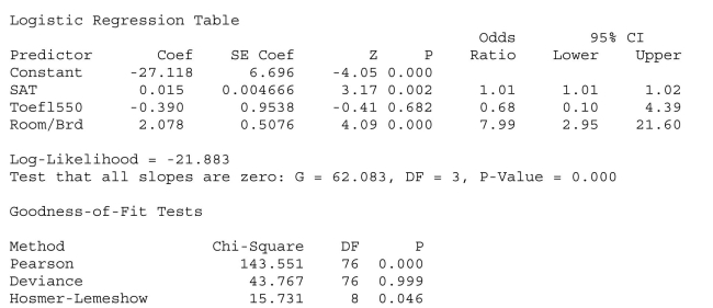-Referring to Scenario 18-11, what is the p-value of the test statistic when testing whether SAT makes a significant contribution to the model in the presence of the other independent variables?

It was believed that the probability of being hit by lightning is the same during the course of a thunderstorm.Which of the following distributions would you use to determine the probability of being hit by a lightning during the first half of a thunderstorm?

SCENARIO 18-5 You worked as an intern at We Always Win Car Insurance Company last summer.You notice that individual car insurance premiums depend very much on the age of the individual, the number of traffic tickets received by the individual, and the population density of the city in which the individual lives.You performed a regression analysis in EXCEL and obtained the following information: Regression Analysis -Referring to Scenario 18-5, the multiple regression model is significant at a 10% level of significance.

SCENARIO 18-8 The superintendent of a school district wanted to predict the percentage of students passing a sixth-grade proficiency test.She obtained the data on percentage of students passing the proficiency test (% Passing), daily mean of the percentage of students attending class (% Attendance), mean teacher salary in dollars (Salaries), and instructional spending per pupil in dollars (Spending)of 47 schools in the state. Following is the multiple regression output with as the dependent variable, -Referring to Scenario 18-8, there is sufficient evidence that the percentage of students passing the proficiency test depends on at least one of the explanatory variables at a 5% level of significance.

SCENARIO 18-9 What are the factors that determine the acceleration time (in sec.)from 0 to 60 miles per hour of a car? Data on the following variables for 171 different vehicle models were collected: Accel Time: Acceleration time in sec. Cargo Vol: Cargo volume in cu.ft. HP: Horsepower MPG: Miles per gallon SUV: 1 if the vehicle model is an SUV with Coupe as the base when SUV and Sedan are both 0 Sedan: 1 if the vehicle model is a sedan with Coupe as the base when SUV and Sedan are both 0 The regression results using acceleration time as the dependent variable and the remaining variables as the independent variables are presented below. SCENARIO 18-9 cont. 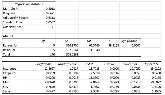The various residual plots are as shown below. 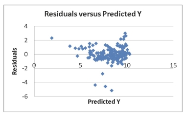SCENARIO 18-9 cont. 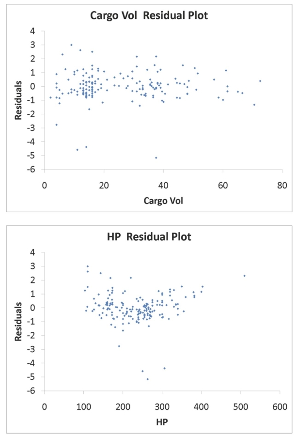SCENARIO 18-9 cont. The coefficient of partial determination of each of the 5 predictors are, respectively, 0.0380, 0.4376, 0.0248, 0.0188, and 0.0312. The coefficient of multiple determination for the regression model using each of the 5 variables as the dependent variable and all other X variables as independent variables ( )are, respectively, 0.7461, 0.5676, 0.6764, 0.8582, 0.6632. -Referring to Scenario 18-9, there is enough evidence to conclude that HP makes a significant contribution to the regression model in the presence of the other independent variables at a 5% level of significance.

SCENARIO 18-11 A logistic regression model was estimated in order to predict the probability that a randomly chosen university or college would be a private university using information on mean total Scholastic Aptitude Test score (SAT)at the university or college, the room and board expense measured in thousands of dollars (Room/Brd), and whether the TOEFL criterion is at least 550 (Toefl550 = 1 if yes, 0 otherwise.)The dependent variable, Y, is school type (Type = 1 if private and 0 otherwise). The Minitab output is given below: -Referring to Scenario 18-11, what is the p-value of the test statistic when testing whether the model is a good-fitting model?

A survey was conducted to determine how people rated the quality of programming available on television.Respondents were asked to rate the overall quality from 0 (no quality at all)to 100 (extremely good quality).A cumulative percentage polygon (ogive) can be used to present this information.