Exam 16: Regression Analysis: Model Building
Exam 1: Data and Statistics85 Questions
Exam 2: Descriptive Statistics: Tabular and Graphical Displays112 Questions
Exam 3: Descriptive Statistics: Numerical Measures139 Questions
Exam 4: Introduction to Probability129 Questions
Exam 5: Discrete Probability Distributions150 Questions
Exam 6: Continuous Probability Distributions144 Questions
Exam 7: Sampling and Sampling Distributions119 Questions
Exam 8: Interval Estimation118 Questions
Exam 9: Hypothesis Tests118 Questions
Exam 10: Inference About Means and Proportions With Two Populations127 Questions
Exam 11: Inferences About Population Variances113 Questions
Exam 12: Tests of Goodness of Fit, Independence and Multiple Proportions76 Questions
Exam 13: Experimental Design and Analysis of Variance125 Questions
Exam 14: Simple Linear Regression103 Questions
Exam 15: Multiple Regression109 Questions
Exam 16: Regression Analysis: Model Building82 Questions
Exam 17: Time Series Analysis and Forecasting80 Questions
Exam 18: Nonparametric Methods83 Questions
Exam 19: Statistical Methods for Quality Control75 Questions
Exam 20: Decision Analysis71 Questions
Exam 21: Sample Survey68 Questions
Select questions type
Consider the following data.  Use Excel's Regression Tool to estimate a second-order model of the form
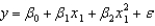
(Essay)
4.7/5  (25)
(25)
Consider the following data.  Use Excel's Regression Tool to estimate a general linear model of the form
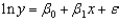
(Essay)
4.8/5 (27)
The variable selection procedure that identifies the best regression equation, given a specified number of independent variables, is
(Multiple Choice)
4.9/5 (36)
Consider the following data.  a.Draw a scatter diagram. Does the relationship between x and y appear to be linear?
b.Assume the relationship between x and y can best be given by
y = 0 + 1+
Estimate the parameters of this curvilinear function.
a.Draw a scatter diagram. Does the relationship between x and y appear to be linear?
b.Assume the relationship between x and y can best be given by
y = 0 + 1+
Estimate the parameters of this curvilinear function.
(Essay)
4.9/5 (34)
Exhibit 16-2
In a regression model involving 30 observations, the following estimated regression equation was obtained.  = 170 + 34x1 - 3x2 + 8x3 + 58x4 + 3x5
For this model, SSR = 1,740 and SST = 2,000.
-Refer to Exhibit 16-2. The coefficient of determination for this model is
= 170 + 34x1 - 3x2 + 8x3 + 58x4 + 3x5
For this model, SSR = 1,740 and SST = 2,000.
-Refer to Exhibit 16-2. The coefficient of determination for this model is
(Multiple Choice)
4.9/5 (28)
Consider the following data.  Use Excel's Regression Tool to estimate a general linear model of the form
(Essay)
4.9/5 (33)
A regression model relating the yearly income (y), age (x1), and the gender of the faculty member of a university (x2 = 1 if female and 0 if male) resulted in the following information.  = 5,000 + 1.2x1 + 0.9x2
n = 20 SSE = 500 SSR = 1,500
Sb1 = 0.2 Sb2 = 0.1
a.Is gender a significant variable?
b.Determine the multiple coefficient of determination.
= 5,000 + 1.2x1 + 0.9x2
n = 20 SSE = 500 SSR = 1,500
Sb1 = 0.2 Sb2 = 0.1
a.Is gender a significant variable?
b.Determine the multiple coefficient of determination.
(Short Answer)
4.9/5 (40)
Exhibit 16-2
In a regression model involving 30 observations, the following estimated regression equation was obtained. = 170 + 34x1 - 3x2 + 8x3 + 58x4 + 3x5
For this model, SSR = 1,740 and SST = 2,000.
-Refer to Exhibit 16-2. The value of SSE is
(Multiple Choice)
4.9/5 (27)
The following regression model y = 0 + 1x1 + 2x2 +
Is known as
(Multiple Choice)
4.7/5 (39)
We are interested in determining what type of model best describes the relationship between two variables x and y.
a.For a given data set, an estimated regression equation relating x and y of the formwas developed, using Excel. The results are shown below. Comment on the adequacy of this equation for predicting y. Let = .05. 
 b.An estimated regression equation for the same data set (as in part a) of the formwas developed. The Excel output is shown below. Comment on the adequacy of this equation for predicting y. Let = .05.
  c.Use the results of Part b and predict y when x = 4.
(Essay)
4.9/5 (32)
Exhibit 16-4
In a laboratory experiment, data were gathered on the life span (y in months) of 33 rats, units of daily protein intake (x1), and whether or not agent x2 (a proposed life extending agent) was added to the rats diet (x2 = 0 if agent x2 was not added, and x2 = 1 if agent was added.) From the results of the experiment, the following regression model was developed.  = 36 + 0.8x1 - 1.7x2
Also provided are SSR = 60 and SST = 180.
-Refer to Exhibit 16-4. The model
= 36 + 0.8x1 - 1.7x2
Also provided are SSR = 60 and SST = 180.
-Refer to Exhibit 16-4. The model
(Multiple Choice)
4.9/5 (31)
Which of the following statements about the backward elimination procedure is false?
(Multiple Choice)
4.7/5 (32)
Multiple regression analysis was used to study the relationship between a dependent variable, y, and four independent variables; x1, x2, x3 and, x4. The following is a partial result of the regression analysis involving 31 observations.  a.Compute the coefficient of determination.
b.At = 0.05, perform an F test and determine whether or not the regression model is significant.
c.Perform a t test and determine whether or not 1 is significantly different from zero ( = 0.05).
d.Perform a t test and determine whether or not 4 is significantly different from zero ( = 0.05).
a.Compute the coefficient of determination.
b.At = 0.05, perform an F test and determine whether or not the regression model is significant.
c.Perform a t test and determine whether or not 1 is significantly different from zero ( = 0.05).
d.Perform a t test and determine whether or not 4 is significantly different from zero ( = 0.05).
(Essay)
5.0/5 (34)
Exhibit 16-2
In a regression model involving 30 observations, the following estimated regression equation was obtained. = 170 + 34x1 - 3x2 + 8x3 + 58x4 + 3x5
For this model, SSR = 1,740 and SST = 2,000.
-Refer to Exhibit 16-2. The value of MSR is
(Multiple Choice)
5.0/5 (29)
The forward selection procedure starts with how many independent variable(s) in the multiple regression model?
(Multiple Choice)
4.8/5 (34)
Part of an Excel output relating y (dependent variable) and 4 independent variables, x1 through x4, is shown below.  a.Fill in all the blanks marked with "?"
b.At a 5% significance level, which independent variables are significant and which ones are not? Fully explain how you arrived at your answers.
a.Fill in all the blanks marked with "?"
b.At a 5% significance level, which independent variables are significant and which ones are not? Fully explain how you arrived at your answers.
(Essay)
4.8/5 (43)
Exhibit 16-3
Below you are given a partial Excel output based on a sample of 25 observations.  -Refer to Exhibit 16-3. The critical t value obtained from the table to test an individual parameter at the 5% level is
(Multiple Choice)
4.7/5 (34)
Exhibit 16-1
In a regression analysis involving 25 observations, the following estimated regression equation was developed.  = 10 - 18x1 + 3x2 + 14x3
Also, the following standard errors and the sum of squares were obtained.Sb1 = 3 Sb2 = 6 Sb3 = 7
SST = 4,800 SSE = 1,296
-Refer to Exhibit 16-1. The multiple coefficient of determination is
= 10 - 18x1 + 3x2 + 14x3
Also, the following standard errors and the sum of squares were obtained.Sb1 = 3 Sb2 = 6 Sb3 = 7
SST = 4,800 SSE = 1,296
-Refer to Exhibit 16-1. The multiple coefficient of determination is
(Multiple Choice)
4.8/5 (27)
Exhibit 16-2
In a regression model involving 30 observations, the following estimated regression equation was obtained. = 170 + 34x1 - 3x2 + 8x3 + 58x4 + 3x5
For this model, SSR = 1,740 and SST = 2,000.
-Refer to Exhibit 16-2. The degrees of freedom associated with SSE are
(Multiple Choice)
4.9/5 (34)
Exhibit 16-1
In a regression analysis involving 25 observations, the following estimated regression equation was developed. = 10 - 18x1 + 3x2 + 14x3
Also, the following standard errors and the sum of squares were obtained.Sb1 = 3 Sb2 = 6 Sb3 = 7
SST = 4,800 SSE = 1,296
-Refer to Exhibit 16-1. The coefficient of x2
(Multiple Choice)
4.7/5 (32)
Filters
- Essay(0)
- Multiple Choice(0)
- Short Answer(0)
- True False(0)
- Matching(0)